6 Regularization and Penalized Models

Complex models increase the chance of overfitting to the training sample. This leads to:

Poor prediction
Burdensome prediction models for implementation (need to measure lots of predictors)
Low power to test hypothesis about predictor effects

Complex models are difficult to interpret

Regularization is technique that:

Reduces overfitting
Allows for p >> n
May yield more interpretable models (LASSO, Elastic Net)
May reduce implementation burden (LASSO, Elastic Net)

Regularization does this by applying a penalty to the parametric model coefficients (parameter estimates)

This constrains/shrinks these coefficients to yield a simpler/less overfit model

Some types of penalties shrink the coefficients to zero (feature selection)

We will consider three approaches to regularization

$L_2$ (Ridge)
$L_1$ (LASSO)
Elastic net

These approaches are available for both regression and classification problems and for a variety of parametric statistical models

6.1 Cost functions

To understand regularization, we need to first explicitly consider loss/cost functions for the parametric statistical models we have been using.

A loss function quantifies the error between a single predicted and observed outcome within some statistical model.

A cost function is simply the aggregate of the loss across all observations in the training sample.

Optimization procedures (least squares, maximum likelihood, gradient descent) seek to determine a set of parameter estimates that minimize some specific cost function for the training sample.

The cost function for the linear model is the mean squared error (squared loss):

$\frac{1}{n}\sum_{i = 1}^{n} (Y_i - \hat{Y_i})^{2}$

No constraints or penalties are placed on the parameter estimates ($\beta_k$)

They can take on any values with the only goal to minimize the MSE in the training sample

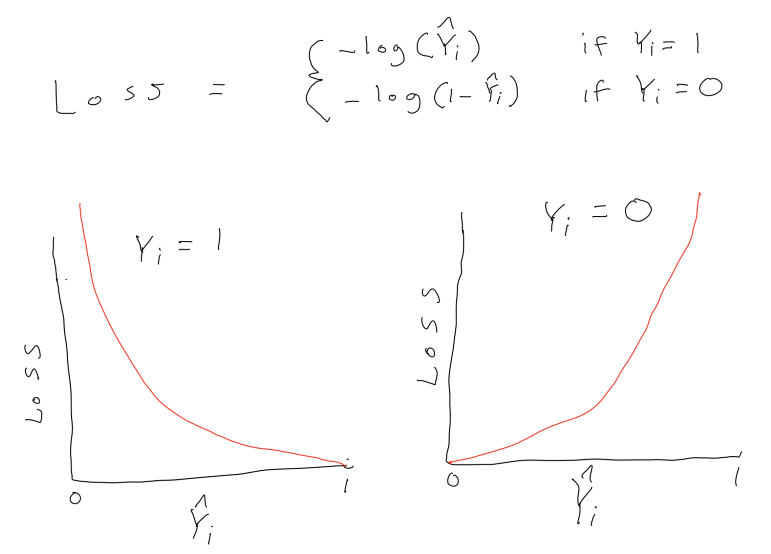
The cost function for logistic regression is log loss:

$\frac{1}{n}\sum_{i = 1}^{n} -Y_ilog(\hat{Y_i}) - (1-Y_i)log(1-\hat{Y_i})$

where $Y_i$ is coded 0,1 and $\hat{Y_i}$ is the predicted probability that Y = 1

Again, no constraints or penalties are placed on the parameter estimates ($\beta_k$)

They can take on any values with the only goal to minimize the sum of the log loss in the training sample

6.2 Intuitions about Penalized Cost Functions and Regularization

This is an example is from a series of wonderfully clear lectures in a machine learning course by Andrew Ng in Coursera.

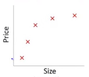
Lets imagine a training set:

House sale price predicted by house size
True DGP is quadratic. Diminishing increase in sale price as size increases
N = 5 in training set

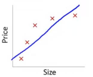
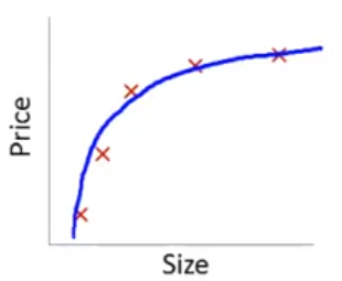
If we fit a linear model with size as the only predictor…

\[\hat{Y_i} = \beta_0 + \beta_1 * size\] In this training set, we might get the following model (in blue)

This is a biased model (predicts too high for low and high house sizes; predicts too low for moderate size houses)

If we took this model to new data from the same quadratic DGP, it would clearly not predict very well

Lets consider the other extreme

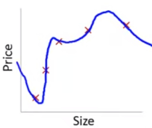
If we fit a 4th order polynomial model using size…

\[\hat{Y_i} = \beta_0 + \beta_1 * size + \beta_2 * size^2 + \beta_3 * size^3 + \beta_4 * size^4\]

In this training set, we would get the following model (in blue)

This is model is overfit to this training set. It would not predict well in new data from the same quadratic DGP

Also, the model would have high variance (if we estimated the parameters in another N = 5 training set, they would be very different)

This problem with overfitting and variance isnt limited to polynomial regression.

We would have the same problem (perfect fit in training with poor fit in new test data) if we predicted housing prices with many predicting when the training N = 5. e.g. -

\[\hat{Y_i} = \beta_0 + \beta_1 * size + \beta_2 * year\_built + \beta_3 * num\_garages + \beta_4 * quality\]

Obviously, the correct model to fit is a second order polynomial model with size

\[\hat{Y_i} = \beta_0 + \beta_1 * size + \beta_2 * size^2\]

But we couldn’t know this with real data because we wouldn’t know the underlying DGP

When we dont know the underlying DGP, we need to be able to consider potentially complex models with many predictors in some way that diminishes the potential problem with overfitting/model variance

Lets consider this intuition:

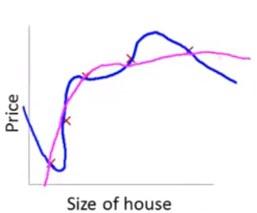
What if we still fit a fourth order polynomial but changed the cost function to penalize the absolute value of $\beta_3$ and $\beta_4$ parameter estimates?

Typical cost based on MSE/squared loss:

$\frac{1}{n}\sum_{i = 1}^{n} (Y_i - \hat{Y_i})^{2}$

Our new cost function:

$[\frac{1}{n}\sum_{i = 1}^{n} (Y_i - \hat{Y_i})^{2}] + [1000 * \beta_3 + 1000 * \beta_4]$

The only way to make the value of this new cost function small is to make $\beta_3$ and $\beta_4$ small

If we made the penalty applied to $\beta_3$ and $\beta_4$ was large (e.g., 1000 as above), we will end up with the parameter estimates for these two features at approximately 0.

With a sufficient penalty applied, their parameter estimates will only change from zero to the degree that these changes accounted for a large enough drop in MSE to offset this penalty in the overall aggregate cost function.

$[\sum_{i = 1}^{n} (Y_i - \hat{Y_i})^{2}] + 1000 * \beta_3 + 1000 * \beta_4$

With this penalty in place, our final model might shift from the blue model to the pink model below. The pink model is mostly quadratic but with a few extra “wiggles” if $\beta_3$ and $\beta_4$ are not exactly 0.

Of course, we dont typically know in advance which parameter estimates to penalize.

Instead, we apply some penalty to all the parameter estimates (except $\beta_0$)

This shrinks the parameter estimates for all the predictors to some degree

However, predictors that do reduce MSE meaningfully will be “worth” including with non-zero parameter estimates

You can also control the shrinkage by controlling the size of the penalty

In general, regularization produces models that:

Are simpler (e.g. smoother, smaller coefficients/parameter estimates)
Are less prone to overfitting
Allow for models with p >> n
Are sometimes more interpretable (LASSO, Elastic Net)

These benefits are provided by the introduction of some bias into the parameter estimates

This allows for a bias-variance trade-off where some bias is introduced for a big reduction in variance of model fit

We will now consider three regularization approaches that introduce different types of penalties to shrink the parameter estimates

$L_2$ (Ridge)
$L_1$ (LASSO)
Elastic net

These approaches are available for both regression and classification problems and for a variety of parametric statistical models

A fourth common regularized classification model (also sometimes used for regression) is the support vector machine

Each of these approaches uses a different specific penalty, which has implications for how the model performs in different settings

6.3 Ridge Regression

The cost function for Ridge Regression is:

\[\frac{1}{n}([\sum_{i = 1}^{n} (Y_i - \hat{Y_i})^{2}] + [\:\lambda\sum_{j = 1}^{p} \beta_j^{2}\:])\] It has two components:

Inside the left brackets is the SSE from linear regression
Inside the right brackets is the Ridge penalty. This penalty:
- Includes the sum of the squared parameter estimates (excluding $\beta_0$). Squaring removes the sign of these parameter estimates.
- This sum is multiplied by $\lambda$, a hyperparameter in Ridge regression. Lambda allows us to tune the size of the penalty.
- This is an application of the $L_2$ norm to the vector of parameter estimates

\[\frac{1}{n}([\sum_{i = 1}^{n} (Y_i - \hat{Y_i})^{2}] + [\:\lambda\sum_{j = 1}^{p} \beta_j^{2}\:])\]

What will happen to a Ridge regression model’s parameter estimates and its performance (i.e., its bias & variance) as lambda increases/decreases?

What is the special case of Ridge regression when lambda = 0?

Lets compare Ridge regression to OLS (ordinary least squares with squared loss cost function) linear regression

Ridge parameter estimates are biased but have lower variance (smaller SE) than OLS
Ridge may predict better in new data
- This depends on the value of $\lambda$ selected and its impact on bias-variance trade-off in Ridge regression vs. OLS)
- There does exist a value of $\lambda$ for which Ridge predicts better than OLS in new data
Ridge regression (but not OLS) allows for p > (or even >>) than n
Ridge regression (but not OLS) accomodates highly correlated (or even perfectly multi-collinear) predictors
OLS (but not Ridge regression) is scale invariant
- You should scale (mean and standard deviation correct) predictors for use with Ridge regression

\[\frac{1}{n}([\sum_{i = 1}^{n} (Y_i - \hat{Y_i})^{2}] + [\:\lambda\sum_{j = 1}^{p} \beta_j^{2}\:])\]

Why does the scale of the predictors matter for Ridge regression?

Unless the predictors are on the same scale to start, you should standardize them for all applications (regression and classification) of Ridge (and also LASSO and elastic net). You should do this explicitly in Caret.
Y should also be standardized for Ridge, LASSO, and elastic net for regression problems with Gaussian distribution for Y. Caret will do this automatically for you.

6.4 LASSO Regression

LASSO is an acronym for Least Absolute Shrinkage and Selection Operator

The cost function for LASSO Regression is:

\[\frac{1}{n}([\sum_{i = 1}^{n} (Y_i - \hat{Y_i})^{2}] + [\:\lambda\sum_{j = 1}^{p} |\beta_j|\:])\] It has two components:

Inside the left brackets is the SSE from linear regression
Inside the right brackets is the LASSO penalty. This penalty:
- Includes the sum of the absolute value of the parameter estimates (excluding $\beta_0$). The absolute value removes the sign of these parameter estimates.
- This sum is multiplied by $\lambda$, a hyperparameter in LASSO regression. Lambda allows us to tune the size of the penalty.
- This is an application of the $L_1$ norm to the vector of parameter estimates

6.5 LASSO vs. Ridge Comparison

With respect to the parameter estimates:

LASSO yields sparse solution (some parameter estimates set to exactly zero)
Ridge tends to retain all predictors (parameter estimates don’t get set to exactly zero)
LASSO selects one predictor among correlated group and sets others to zero
Ridge shrinks all parameter estimates for correlated predictors

Neither LASSO nor Ridge perform systematically better than the other across all contexts

Advantages of LASSO

Does feature selection (sets parameter estimates to exactly 0)
- Yields a sparse solution
- Sparse model is more interpretable?
- Sparse model is easier to implement? (fewer predictors included so don’t need to measure as many)
More robust to outliers (similar to LAD vs. OLS)
Tends to do better when there are a small number of significant predictors and the others are close to zero or zero

Advantages of Ridge

Computationally superior (closed form solution vs. iterative; Only one solution to minimize the cost function)
More robust to measurement error in predictors
Tends to do better when there are many predictors with large (and comparable) effects (i.e., most predictors are related to the outcome)

6.6 Elastic Net Regression

The Elastic Net blends the $L_1$ and $L_2$ penalties to obtain the benefits of each of those approaches.

We will use the implementation of the Elastic Net in glmnet in R.

You can also read additional introductory documentation for this package

In the Gaussian regression context, the Elastic Net cost function is:

\[\frac{1}{n}([\sum_{i = 1}^{n} (Y_i - \hat{Y_i})^{2}] + [\:\lambda (\alpha\sum_{j = 1}^{p} |\beta_j| + (1-\alpha)\sum_{j = 1}^{p} \beta_j^{2})\:])\]

This model has two hyper-parameters

$\lambda$ controls the degree of regularization as before
$\alpha$ is a “mixing” parameter that blends the degree of $L_1$ and $L_2$ contributions to the aggregate penalty
- $\alpha$ = 1 results in the LASSO model
- $\alpha$ = 0 results in the Ridge model
- Intermediate values for $\alpha$ blend these penalties together proportionally

6.7 Hyper-parameter Selection

As before (e.g., KNN), best values of $\lambda$ (and $\alpha$) can be selected using cross validation

Depending on your goals and the model, you can use $tuneLength$ or $tuneGrid$

If you use $tuneGrid$, you have to choose good values for $\lambda$. $glmnet$ has methods for selecting good values (more on this in example)

6.8 Applications in a Sample Dataset

Lets make a dataset you might find in an explanatory setting in Psychology

A focal dichotomous IV (x; your experimental manipulation)
A number of covariates (some good, some not so good)
A quantitative outcome (y)

NOTES:

x and covariates are uncorrelated
covariates are uncorrelated (use $mvrnorm()$ for correlated variables)
DGP" y is a linear function of x, good_ covs and normally distributed (via $rnorm()$) noise

library(caret)
library(tidyverse)
library(doParallel)

#settings
n <- 120
n_good_covs <- 4
n_bad_covs <- 8
eff_x <- .3
eff_good_covs <- .4
noise <- 1

effs <- matrix(c(eff_x, rep(eff_good_covs, n_good_covs), rep(0, n_bad_covs)), ncol = 1)
varnames <- c(str_c("good_cov", 1:n_good_covs), str_c("bad_cov", 1:n_bad_covs))
n_covs <- n_good_covs + n_bad_covs

set.seed(123456)
d <- matrix(rnorm(n * n_covs), nrow = n, dimnames = list(NULL, varnames)) %>% 
  as_tibble() %>% 
  mutate(x = rep(c(-.5,.5), n/2)) %>% 
  select(x, everything()) %>% 
  mutate(y = rnorm(n, (as.matrix(.) %*% effs), noise)) %>% 
  select(y, everything())

Here are the correlations with y in THIS specific sample:

#corrs with y
cor(d)[,1]

##            y            x    good_cov1    good_cov2    good_cov3    good_cov4     bad_cov1 
##  1.000000000  0.229494369  0.354540653  0.333808148  0.399702925  0.304823392 -0.064352306 
##     bad_cov2     bad_cov3     bad_cov4     bad_cov5     bad_cov6     bad_cov7     bad_cov8 
## -0.027858626  0.054200073  0.004900236  0.015368822  0.009046430  0.062775162 -0.063284139

Now lets get all_x and all_y for training

all_x <- d %>% 
  select(-y) %>% 
  as.data.frame()

all_y <- d %>% 
  pull(y)

Lets consider how you might test the effect of x in a traditional GLM

You want to use covariates to increase power
BUT you don’t know which covariates to use
You might use all of them
Or you might use none of them (a clear lost opportunity)
Or you might hack it by using those increase your focal x effect (very bad!)

Lets evaluate this model and the effect of x using all covariates

Set up $trainControl()$
Set up parallel processing

tc_kfold <- trainControl(method = "cv", number = 10, 
                         savePredictions = TRUE)

(n_core <- detectCores())

## [1] 8

if(n_core > 2) {
  cl <- makeCluster(n_core - 1, outfile = "")
  registerDoParallel(cl)
  getDoParWorkers()
}

## [1] 7

You want the GLM fit in the full sample to test x effect

You want the GLM evaluated via CV to see its performance in held-out data

$train()$ paired with the previous $trainControl()$ will do both

m_glm <- train(x = all_x, y = all_y, 
                     method = "glm",
                     trControl = tc_kfold, 
                     tuneLength = 10,
                     metric = "RMSE")

m_glm

## Generalized Linear Model 
## 
## 120 samples
##  13 predictor
## 
## No pre-processing
## Resampling: Cross-Validated (10 fold) 
## Summary of sample sizes: 108, 108, 108, 108, 108, 108, ... 
## Resampling results:
## 
##   RMSE      Rsquared   MAE     
##   1.070695  0.4011136  0.872425

The model has an RMSE of 1.0706952 in held-out data (via k-fold)

You can see more or less detail in various ways

m_glm$results

##   parameter     RMSE  Rsquared      MAE    RMSESD RsquaredSD     MAESD
## 1      none 1.070695 0.4011136 0.872425 0.2603685  0.1980792 0.1963452

m_glm$resample

##         RMSE   Rsquared       MAE Resample
## 1  0.7180025 0.71704296 0.6119957   Fold01
## 2  1.0811150 0.59405315 0.8505256   Fold02
## 3  1.1448330 0.09374476 0.9481425   Fold03
## 4  1.4434445 0.25527693 1.2021417   Fold04
## 5  1.3636814 0.51517066 1.0063702   Fold05
## 6  1.1372802 0.31181692 0.8992346   Fold06
## 7  0.8935512 0.20211990 0.7389951   Fold07
## 8  1.3271614 0.28773253 1.0994530   Fold08
## 9  0.7439114 0.51689623 0.6338409   Fold09
## 10 0.8539710 0.51728236 0.7335505   Fold10

Remember, we generated y using this DGP:

$y = rnorm(n, x * effs, noise)$

What is the irreducible error for this model? In other words, if we developed a model where there was no bias in the coefficients and no overfitting, what should the RMSE of that model be?

Lets look at model coefficients and test x

Model has 14 non-zero parameter estimates (including $\beta_0$)

Critically, the coefficients for bad covariates range from -0.2035268 and 0.1100836

These coefficients are overfit to this sample, predicting noise in this sample that will not be present in the same form in new data

coef(m_glm$finalModel)

##  (Intercept)            x    good_cov1    good_cov2    good_cov3    good_cov4     bad_cov1 
##  0.040875810  0.290659481  0.516014221  0.380294334  0.534015168  0.404416218 -0.082317462 
##     bad_cov2     bad_cov3     bad_cov4     bad_cov5     bad_cov6     bad_cov7     bad_cov8 
## -0.203526763 -0.009054937  0.013163329 -0.068502231  0.110083599  0.048444108 -0.052478450

summary(m_glm)

## 
## Call:
## NULL
## 
## Deviance Residuals: 
##      Min        1Q    Median        3Q       Max  
## -2.05638  -0.65725  -0.00638   0.59984   2.90664  
## 
## Coefficients:
##              Estimate Std. Error t value Pr(>|t|)    
## (Intercept)  0.040876   0.098001   0.417 0.677453    
## x            0.290659   0.196516   1.479 0.142089    
## good_cov1    0.516014   0.099912   5.165 1.14e-06 ***
## good_cov2    0.380294   0.100166   3.797 0.000245 ***
## good_cov3    0.534015   0.093380   5.719 1.00e-07 ***
## good_cov4    0.404416   0.095346   4.242 4.76e-05 ***
## bad_cov1    -0.082317   0.104095  -0.791 0.430831    
## bad_cov2    -0.203527   0.105180  -1.935 0.055650 .  
## bad_cov3    -0.009055   0.091581  -0.099 0.921426    
## bad_cov4     0.013163   0.101337   0.130 0.896895    
## bad_cov5    -0.068502   0.087667  -0.781 0.436316    
## bad_cov6     0.110084   0.096413   1.142 0.256115    
## bad_cov7     0.048444   0.095571   0.507 0.613282    
## bad_cov8    -0.052478   0.092250  -0.569 0.570644    
## ---
## Signif. codes:  0 '***' 0.001 '**' 0.01 '*' 0.05 '.' 0.1 ' ' 1
## 
## (Dispersion parameter for gaussian family taken to be 1.010856)
## 
##     Null deviance: 221.03  on 119  degrees of freedom
## Residual deviance: 107.15  on 106  degrees of freedom
## AIC: 356.95
## 
## Number of Fisher Scoring iterations: 2

Regression and classification models with Ridge, LASSO, and Elastic Net penalties are easily implemented in caret with method = “glmnet”.

If you are fitting an Elastic Net, I recommend letting glmnet (through caret) choose the values of the hyper-parameters to select among during model tuning. Simply specify $tuneLength$.

Here it selects a crossing of up to 10 values of $\lambda$ and 10 values of $\alpha$

$glmnet$ does “warm-starts” when training models with different hyper-parameters. It can train all of these 100 models across hyperparamters within one resample almost as fast as it can train one single set of hyperparameters

m_net <- train(x = all_x, y = all_y, 
                     method = "glmnet",
                     trControl = tc_kfold, 
                     tuneLength = 10,
                     metric = "RMSE",
                     preProcess = c("center", "scale", "nzv"))

m_net

## glmnet 
## 
## 120 samples
##  13 predictor
## 
## Pre-processing: centered (13), scaled (13) 
## Resampling: Cross-Validated (10 fold) 
## Summary of sample sizes: 108, 108, 108, 108, 108, 108, ... 
## Resampling results across tuning parameters:
## 
##   alpha  lambda       RMSE      Rsquared   MAE      
##   0.1    0.001337543  1.049648  0.4498276  0.8688818
##   0.1    0.003089898  1.049648  0.4498276  0.8688818
##   0.1    0.007138066  1.049482  0.4498623  0.8687614
##   0.1    0.016489858  1.047418  0.4505810  0.8671588
##   0.1    0.038093711  1.043087  0.4522084  0.8635134
##   0.1    0.088001415  1.035706  0.4554110  0.8577880
##   0.1    0.203294687  1.030245  0.4596085  0.8494807
##   0.1    0.469637106  1.044163  0.4659696  0.8579125
##   0.2    0.001337543  1.049563  0.4499517  0.8687394
##   0.2    0.003089898  1.049563  0.4499517  0.8687394
##   0.2    0.007138066  1.048949  0.4501678  0.8682626
##   0.2    0.016489858  1.046195  0.4513074  0.8659326
##   0.2    0.038093711  1.040622  0.4537063  0.8610679
##   0.2    0.088001415  1.032292  0.4576365  0.8534858
##   0.2    0.203294687  1.029869  0.4623207  0.8497798
##   0.2    0.469637106  1.050914  0.4783592  0.8634588
##   0.3    0.001337543  1.049538  0.4500259  0.8686826
##   0.3    0.003089898  1.049538  0.4500259  0.8686826
##   0.3    0.007138066  1.048405  0.4504842  0.8677262
##   0.3    0.016489858  1.045003  0.4519886  0.8647377
##   0.3    0.038093711  1.038348  0.4550387  0.8588362
##   0.3    0.088001415  1.029918  0.4592381  0.8496421
##   0.3    0.203294687  1.028358  0.4674103  0.8486445
##   0.3    0.469637106  1.065115  0.4874239  0.8759617
##   0.4    0.001337543  1.049554  0.4500573  0.8686667
##   0.4    0.003089898  1.049554  0.4500573  0.8686667
##   0.4    0.007138066  1.047868  0.4507933  0.8671894
##   0.4    0.016489858  1.043838  0.4526619  0.8635367
##   0.4    0.038093711  1.036222  0.4563142  0.8567022
##   0.4    0.088001415  1.028246  0.4606873  0.8478101
##   0.4    0.203294687  1.028520  0.4725960  0.8480291
##   0.4    0.469637106  1.091719  0.4807967  0.8947348
##   0.5    0.001337543  1.049554  0.4500788  0.8686302
##   0.5    0.003089898  1.049447  0.4501131  0.8685508
##   0.5    0.007138066  1.047332  0.4510987  0.8666529
##   0.5    0.016489858  1.042708  0.4532978  0.8623315
##   0.5    0.038093711  1.034608  0.4570381  0.8548045
##   0.5    0.088001415  1.027718  0.4614760  0.8475749
##   0.5    0.203294687  1.030787  0.4769975  0.8496314
##   0.5    0.469637106  1.125254  0.4657795  0.9182151
##   0.6    0.001337543  1.049517  0.4500940  0.8685937
##   0.6    0.003089898  1.049246  0.4502136  0.8683566
##   0.6    0.007138066  1.046795  0.4513965  0.8661302
##   0.6    0.016489858  1.041618  0.4538931  0.8611237
##   0.6    0.038093711  1.033008  0.4579269  0.8527305
##   0.6    0.088001415  1.026115  0.4633213  0.8465010
##   0.6    0.203294687  1.034853  0.4806936  0.8527003
##   0.6    0.469637106  1.162161  0.4454704  0.9430657
##   0.7    0.001337543  1.049588  0.4500775  0.8686356
##   0.7    0.003089898  1.049004  0.4503517  0.8681206
##   0.7    0.007138066  1.046263  0.4516923  0.8656070
##   0.7    0.016489858  1.040555  0.4544801  0.8600646
##   0.7    0.038093711  1.031703  0.4586304  0.8507429
##   0.7    0.088001415  1.024338  0.4659260  0.8456935
##   0.7    0.203294687  1.040943  0.4833126  0.8582490
##   0.7    0.469637106  1.204036  0.4118519  0.9728206
##   0.8    0.001337543  1.049564  0.4501278  0.8686085
##   0.8    0.003089898  1.048764  0.4504864  0.8678842
##   0.8    0.007138066  1.045738  0.4519855  0.8650853
##   0.8    0.016489858  1.039479  0.4550900  0.8590087
##   0.8    0.038093711  1.030623  0.4591923  0.8495190
##   0.8    0.088001415  1.022988  0.4683819  0.8451303
##   0.8    0.203294687  1.049923  0.4824615  0.8662607
##   0.8    0.469637106  1.248240  0.3583697  1.0033596
##   0.9    0.001337543  1.049581  0.4501189  0.8686299
##   0.9    0.003089898  1.048527  0.4506205  0.8676496
##   0.9    0.007138066  1.045219  0.4522767  0.8645617
##   0.9    0.016489858  1.038433  0.4556920  0.8579480
##   0.9    0.038093711  1.029655  0.4597436  0.8483811
##   0.9    0.088001415  1.022251  0.4706079  0.8447612
##   0.9    0.203294687  1.061615  0.4779668  0.8756531
##   0.9    0.469637106  1.287334  0.2736696  1.0278612
##   1.0    0.001337543  1.049546  0.4501229  0.8685658
##   1.0    0.003089898  1.048293  0.4507533  0.8674169
##   1.0    0.007138066  1.044703  0.4525691  0.8640364
##   1.0    0.016489858  1.037558  0.4561010  0.8570617
##   1.0    0.038093711  1.028892  0.4603008  0.8475576
##   1.0    0.088001415  1.022192  0.4724619  0.8449953
##   1.0    0.203294687  1.074783  0.4725416  0.8854512
##   1.0    0.469637106  1.317786  0.1814477  1.0488529
## 
## RMSE was used to select the optimal model using the smallest value.
## The final values used for the model were alpha = 1 and lambda = 0.08800141.

The Elastic Net model has an RMSE of 1.0221917 in held-out data (via k-fold), which is better than the previous GLM (1.0706952).

This, simpler, regularized model that penalized the coefficients to encourage them to remain small:

Increased bias (if you simulated repeated sample from this DGP and fit models to each sample, the coefficients would not average to their population values)
Decreased overfitting leading to less variance

m_net$resample  #resample results for best hyper-parameter

##         RMSE  Rsquared       MAE Resample
## 1  1.5379109 0.2748093 1.3484846   Fold01
## 2  1.0599903 0.5793474 0.8963869   Fold06
## 3  0.7371125 0.7583896 0.5687542   Fold03
## 4  1.0204921 0.5947351 0.8632055   Fold09
## 5  0.9325653 0.4270229 0.8334295   Fold10
## 6  1.0562827 0.1575908 0.8763435   Fold08
## 7  1.1391636 0.3967559 0.8134234   Fold07
## 8  0.5889101 0.6337160 0.4185353   Fold05
## 9  1.0588382 0.5710349 0.8957313   Fold04
## 10 1.0906512 0.3312168 0.9356586   Fold02

mean(m_net$resample$RMSE) #mean resample across k folds for best hyper-parameter

## [1] 1.022192

Lets look at the best values of the hyper-parameters that were selected to minimize RMSE in held out data by k-fold CV.

m_net$bestTune

##    alpha     lambda
## 78     1 0.08800141

Looking at the value of these two hyper-parameters, what do you notice?

Let’s look at the model coefficients

CODE NOTE: Use of the second arguement to $coef()$ to get the coefs for the best model (you just need to specify lambda)

coef(m_net$finalModel, m_net$finalModel$lambdaOpt)

## 14 x 1 sparse Matrix of class "dgCMatrix"
##                         1
## (Intercept)  0.0579755763
## x            0.1107473540
## good_cov1    0.4008329642
## good_cov2    0.2911686886
## good_cov3    0.4506804929
## good_cov4    0.3116627094
## bad_cov1     .           
## bad_cov2    -0.0803001895
## bad_cov3     .           
## bad_cov4     .           
## bad_cov5     .           
## bad_cov6     0.0005987057
## bad_cov7     .           
## bad_cov8     .

The Elastic Net penalty set the parameter estimate for most of the bad_covs to exactly zero. That is likely why this model is less overfit than the GLM and predicts better in new data.

However, the parameter estimate for x is also biased. Notice its value (you cant tell its biased from one sample, but it would repeatedly be smaller than it should be because of this bias.

In some explanatory situation, you might consider not penalizing the parameter estimate for x

This would allow you to fit the best covariate model but still retain a possibly unbiased estimate of x

This would make most sense in a situation where x was manipulated and therefore uncorrelated with the covariates

CODE NOTE: $penalty.factor$ is argument in $glmnet$. Passed to $glmnet$ via $...$ argument in $train()$

names(all_x)

##  [1] "x"         "good_cov1" "good_cov2" "good_cov3" "good_cov4" "bad_cov1"  "bad_cov2" 
##  [8] "bad_cov3"  "bad_cov4"  "bad_cov5"  "bad_cov6"  "bad_cov7"  "bad_cov8"

penatly_factor <- if_else(str_detect(names(all_x),"x"), 0,1)
penatly_factor

##  [1] 0 1 1 1 1 1 1 1 1 1 1 1 1

m_net_x <- train(x = all_x, y = all_y, 
                     method = "glmnet",
                     trControl = tc_kfold, 
                     tuneLength = 10,
                     metric = "RMSE",
                     preProcess = c("center", "scale", "nzv"),
                     penalty.factor = penatly_factor)

Lets look at model performance and parameter estimates

Its RMSE (1.0316178) is essentially the same as the model that penalized x (1.0221917)

The parameter estimate for x is now 0.2052717 vs. coef(m_net$finalModel, m_net$finalModel$lambdaOpt)[“x”,1] previously

mean(m_net_x$resample$RMSE)

## [1] 1.031618

coef(m_net_x$finalModel, m_net_x$finalModel$lambdaOpt)

## 14 x 1 sparse Matrix of class "dgCMatrix"
##                       1
## (Intercept)  0.05797558
## x            0.20527170
## good_cov1    0.38234594
## good_cov2    0.27894645
## good_cov3    0.42884106
## good_cov4    0.30543861
## bad_cov1     .         
## bad_cov2    -0.06022389
## bad_cov3     .         
## bad_cov4     .         
## bad_cov5     .         
## bad_cov6     .         
## bad_cov7     .         
## bad_cov8     .

In an explanatory context, you probably want more than a descriptive estimate of the parameter estimate for x

You probably want its SE and a confidence interval

There is not a closed form solution for the SE. We will discuss how to bootstrap an SE estimate in the next unit.

A final CODE NOTE

In most instances, you will want the Elastic Net and allow it to select the values of alpha and lambda to tune over

However if you want to fit a pure Ridge (alpha = 0) or pure LASSO (alpha = 1) model, you will need to specify a $tuneGrid$ rather than use $tuneLength$.

In this instance, you might still want to allow glmnet to select good possible values for lambda

This function will allow you to use glmnet to select good values for lambda

#modified code from Kuhn described here: https://github.com/topepo/caret/issues/116

get_lambdas <- function(x, y, len = 50, model = "LASSO") {
  library(glmnet)
  
  numLev <- if(is.character(y) | is.factor(y)) length(levels(y)) else NA
  
  if(!is.na(numLev)) {
    fam <- ifelse(numLev > 2, "multinomial", "binomial")
  } else fam <- "gaussian" 
  
  if (toupper(model) == "LASSO"){
    alpha <- 1
  } else alpha <- 0
  
  init <- glmnet(as.matrix(x), y, 
                 family = fam, 
                 nlambda = len+2, 
                 alpha = alpha)
  lambda <- unique(init$lambda)
  lambda <- lambda[-c(1, length(lambda))]
  lambda <- lambda[1:min(length(lambda), len)]
}

6.9 Ridge, LASSO, and Elastic net models for other Y distributions

These penalties can be added to the cost functions of other generalized linear models to yield regularized/penalized versions of those models as well

For example

L1 penalized (LASSO) logisitc regression (w/ labels coded 0,1): \[\frac{1}{n}([\:\sum_{i = 1}^{n} -Y_ilog(\hat{Y_i}) - (1-Y_i)log(1-\hat{Y_i})\:]\:+\:[\:\lambda\sum_{j = 1}^{p} |\beta_j|\:] \]
For L2 penalized (Ridge) logisitc regression (w/ labels coded 0,1) \[\frac{1}{n}([\:\sum_{i = 1}^{n} -Y_ilog(\hat{Y_i}) - (1-Y_i)log(1-\hat{Y_i})\:]\:+\:[\:\lambda\sum_{j = 1}^{p} \beta_j^{2}\:] \]

etc…

The full family of these three types of penalties within the GLM is implemented in the $glmnet$ package using $method = "glmnet"$ in $train()$ with caret