5 Subsetting and Univariate Filters
5.1 Unit Overview
Complex models tha that include many predictors increase the chance of overfitting to the training sample. This leads to:
- Poor prediction
- Burdensome prediction models for implementation (need to measure lots of predictors)
- Low power to test hypothesis about predictor effects
Complex models are difficult to intepret
Many parametric models (linear model, generalized linear model, linear discriminant analysis):
- Become very overfit as p approaches n
- Cannot be used when p >= n
- Yet, today we often have p >> n (NLP studies, genetics, precision medicine)
To reduce overfitting and/or allow p >> n, we need methods that can:
- Reduce effective p (select or combine)
- Constrain coefficients
Over the next few units, we will consider three methods to accomplish this:
- Subset selection and filtering approaches (this unit)
- Regularization (penalized models)
- Dimensionality Reduction
5.2 Subset Selection Methods
Subset selection methods involve comparing multiple models that invovle different subsets of predictors to determine the best combination of predictors.
- Best Subset Selection
- Forward Stepwise Selection
- Backward Stepwise Selection
5.3 Best Subset Selection
Let \(M_0\) denote the null model, which contains no predictors. This model simply predicts the sample mean for each observation
For k = 1,2, …, p:
- Fit all models that contain exactly k predictors
- Pick the best among this set of models and call it \(M_k\), Best is defined as having the smallest SSE (or deviance).
Select a single best model from among the \(M_0\), …, \(M_p\) models using cross-validated prediction error or other estimate of test error.
SSE in your training set decreases monotonically with increasing k, but this is constant within a specific k
- Fine to use SSE to compare/select models with same k
- Need to select among models with different k using CV (held-out data)
If you want to evaluate this model, you still need additional held-out data (wrap K-fold CV around this procedure?; single validation set approach?)
These observations are true for all three of the subsetting methods that we will consider in this unit
This approach requires fitting 2p models
- 10 predictors = 1024
- 20 predictors = 1,048,576
- 30 predictors = 1,073,741,824
Best of three approaches when computationally possible
Can be used When p > n: Limit to models up \(M_{n-1}\)
5.4 Forward Stepwise Selection
Let \(M_0\) denote the null model, which contains no predictors.
For k = 0 ,1, …, p-1:
- Consider all p - k models that augment the predictors in \(M_k\) with one additional predictor
- Pick the best among these P-k models and call it \(M_{k+1}\). Best is defined as having the smallest SSE (or deviance).
Select a single best model from among the \(M_0\), …, \(M_p\) models using cross-validated prediction error or other estimate of test error.
This approach requires fitting 1 + p(p+1)/2 models
- 10 predictors = 56
- 20 predictors = 211
- 30 predictors = 466
May miss best model (e.g., \(M_1\) = \(X_1\), but best 2 predictor model should be \(X_2\), \(X_3\). This 2 predictor model is never evaluated because limited to models with \(X_1\))
Can be used When p > n: Limit to models up \(M_{n-1}\)
5.5 Backward Stepwise Selection
Let \(M_p\) denote the full model, which contains all predictors.
For k = p, p-1, 1:
- Consider all k models that contain all but one of the predictors in \(M_k\), for a total of k-1 predictors.
- Pick the best among these k models and call it \(M_{k-1}\). Best is defined as having the smallest SSE (or deviance).
Select a single best model from among the \(M_0\), …, \(M_p\) models using cross-validated prediction error or other estimate of test error.
Like forward stepwise, this approach requires fitting 1 + p(p+1)/2 models
- 10 predictors = 56
- 20 predictors = 211
- 30 predictors = 466
Like forward stepwise, may miss best model.
Backward stepwise requires that n > p because starts with \(M_p\)
However, often better than forward stepwise when both can be used (accounts for unique effects of predictors, controlling for all others)
Methods for choosing the optimal model
- Cross-validation is preferred (makes fewer assumptions and generally computationally feasible?)
- CV can be used with any type of model and with any performance metric
- With GLM (and some other models), you can instead estimate test error by making an adjustment to training error using \(C_p\), AIC, BIC, or Adjusted R2
\(C_p = \frac{1}{n}(SSE + 2p\hat{\sigma}^{2})\)
\(AIC = \frac{1}{n\hat{\sigma}^{2}}(SSE + 2p\hat{\sigma}^{2})\)
\(BIC = \frac{1}{n}(SSE + log(n)p\hat{\sigma}^{2})\)
\(Adusted\:R^2 = 1 - \frac{SSE/(n-p-1)}{SST/(n-1)}\)
\(C_p\), AIC, BIC:
have justifications based on asymptotic arguments (very large n)
converge on same estimate with large n
use with caution with smaller n, not equivalent
- BIC places heavier penalty on models with many predictors; log(n) vs. 2
Adjusted R2 not well justified in statistical theory (but descriptive?)
5.6 Implemention in Caret
There are three main approaches to feature selection:
Regularization (next unit)
Wrapper methods evaluate multiple models using procedures that add and/or remove predictors to find the optimal combination that maximizes model performance. Best subset, forward stepwise and backward stepwise selection are examples of wrapper methods.
Filter methods evaluate the relevance of the predictors outside of the predictive models and subsequently model only the predictors that pass some criterion. I will end with a brief discussion of an implementation of this approach in caret.
Any of the subset approaches we discussed in this unit can be coded manually using for/foreach loops
Kuhn has implemented a robust version of backward stepwise selection that uses cross validation:
- He refers to this as recursive feature elimination
- He has two functions [\(rfe()\) and \(rfeIter()\)] but only \(rfe()\) should be used because it uses a more robust method for selection
- You should read the documentation carefully if you plan to use it
Lets make two very simple datasets with just two IVs and their interaction
You wouldnt need to use subsetting here b/c p << n but the datasets are fine to demo the code and will be useful for class discussion about selecting interactions via subsetting
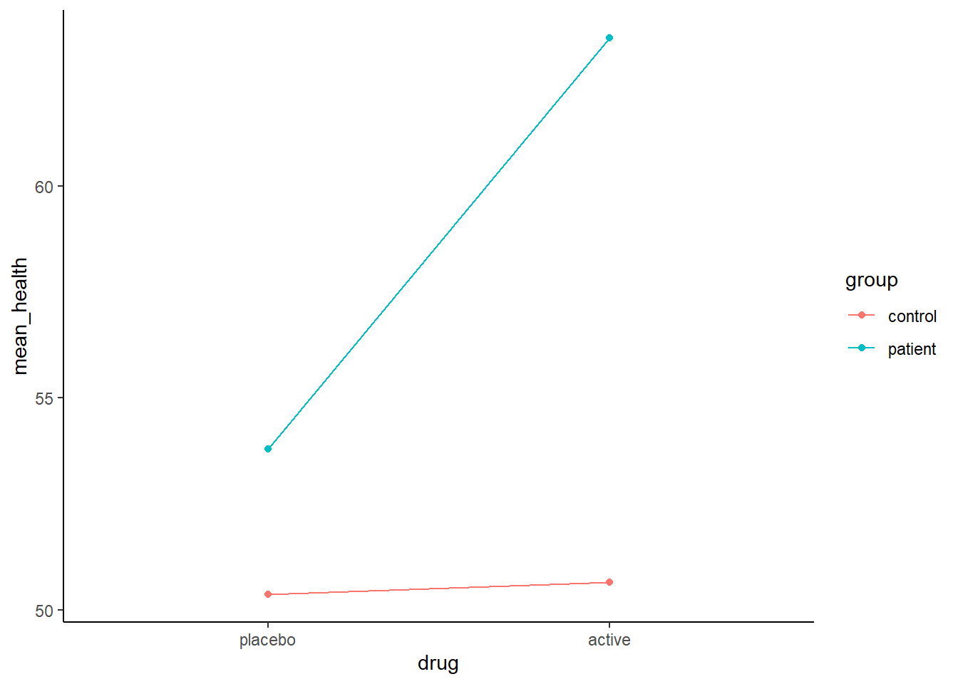
We are modeling health as a function of group (control vs. patient) and drug (placebo vs. active) with normally distributed errors using dummy coded features for both IVs
\(health = 50 + 4 * group + 6 * drug + 10 * group\_x\_drug + \epsilon\)
library(caret)
library(tidyverse)

n <- 1000
group_levels <- c("control", "patient")
drug_levels <- c("placebo", "active")

set.seed(20110522)
d <- tibble(group = rep(group_levels, each = n/2),
              drug = rep(drug_levels, times = n/2)) %>%
  mutate(group = factor(group, levels = group_levels),
         drug = factor(drug, levels = drug_levels))

dmy_codes <- dummyVars(~ group + drug, fullRank = TRUE, sep = "_", data = d)

d <- predict(dmy_codes, d) %>%
  as.data.frame() %>%
  rename(group = group_patient, drug = drug_active) %>%
  mutate(group_x_drug = group * drug,
         health = rnorm(n, 50 + 4 * group + 6 * drug + 10 * group_x_drug, 10))
Here is a plot of the effects in this first simulated data
\(health = 50 + 4 * group + 6 * drug + 10 * group\_x\_drug + \epsilon\)
610/710 REVIEW: Link these coefficients to the graph?

For reference, here is the code that produced this figure
library(ggthemes)
theme_set(theme_classic())
d %>%
  mutate(group = factor(group, labels = group_levels),
         drug = factor(drug, labels = drug_levels)) %>%
  group_by(group, drug) %>%
  summarise(mean_health = mean(health)) %>%
  ggplot() +
  aes(x = drug, y = mean_health, color = group) +
  geom_line(aes(group = group)) +
  geom_point()
Lets use \(rfe()\) to fit a model using backward stepwise selection
x_all <- d %>%
  select(-health)

y_all <- d %>%
  pull(health)

tc <- rfeControl(functions = lmFuncs,
                   method = "repeatedcv",
                   repeats = 5,
                   verbose = FALSE)
subsets = c(1,2,3)
m_rfe1 <- rfe(x = x_all, y = y_all,
                 sizes = subsets,
                 rfeControl = tc)

m_rfe1
##
## Recursive feature selection
##
## Outer resampling method: Cross-Validated (10 fold, repeated 5 times)
##
## Resampling performance over subset size:
##
## Variables RMSE Rsquared MAE RMSESD RsquaredSD MAESD Selected
## 1 10.116 0.3315 8.108 0.6339 0.07950 0.5397
## 2 10.025 0.3434 8.036 0.6634 0.08111 0.5585
## 3 9.964 0.3516 7.941 0.6733 0.08195 0.5547 *
##
## The top 3 variables (out of 3):
## group_x_drug, drug, group## [1] 50 5## Variables RMSE Rsquared MAE Resample
## 3 3 9.660646 0.3483031 7.665247 Fold01.Rep1
## 6 3 10.024831 0.3479045 8.076487 Fold02.Rep1
## 9 3 10.304478 0.3876257 8.128096 Fold03.Rep1
## 12 3 11.206827 0.2829222 9.085973 Fold04.Rep1
## 15 3 9.743766 0.3474785 7.868708 Fold05.Rep1
## 18 3 10.193759 0.3475884 8.150072 Fold06.Rep1## [1] 9.964141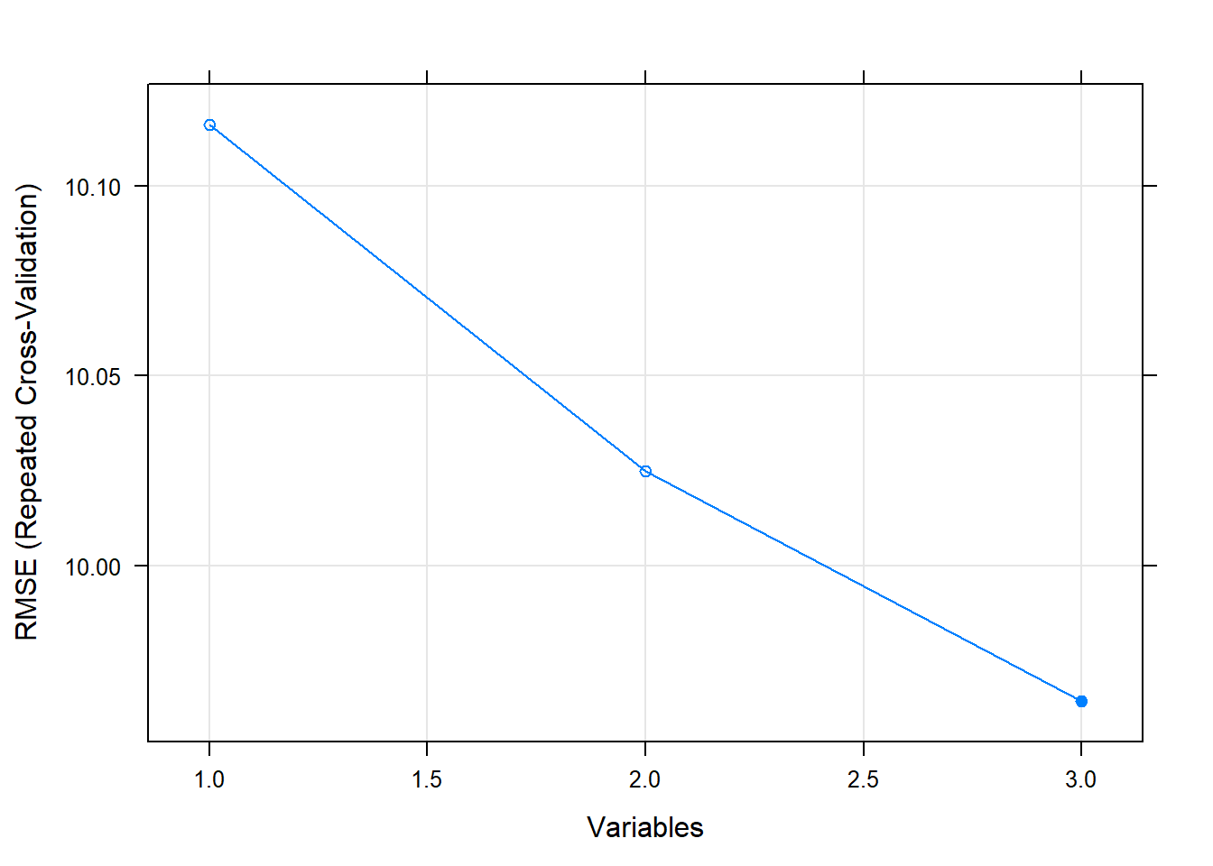
## [1] "group_x_drug" "drug" "group"##
## Call:
## lm(formula = y ~ ., data = tmp)
##
## Coefficients:
## (Intercept) group_x_drug drug group
## 50.693 10.517 5.208 3.434To stimulate class discussion, lets consider another pattern of results with a second simulated dataset
\(health = 50 + 4 * group + 0 * drug + 10 * group\_x\_drug + \epsilon\)
610/710 REVIEW: Link these coefficients to the graph?
d2 <- tibble(group = rep(group_levels, each = n/2),
              drug = rep(drug_levels, times = n/2)) %>%
  mutate(group = factor(group, levels = group_levels),
         drug = factor(drug, levels = drug_levels))

dmy_codes <- dummyVars(~ group + drug, fullRank = TRUE, sep = "_", data = d2)

d2 <- predict(dmy_codes, d2) %>%
  as.data.frame() %>%
  rename(group = group_patient, drug = drug_active) %>%
  mutate(group_x_drug = group * drug,
         health = rnorm(n, 50 + 4 * group + 0 * drug + 10 * group_x_drug, 10))
Here is a plot of the effects in this second simulated data set
\(health = 50 + 4 * group + 0 * drug + 10 * group\_x\_drug + \epsilon\)
Lets use \(rfe()\) again
x_all <- d2 %>%
  select(-health)

y_all <- d2 %>%
  pull(health)

tc <- rfeControl(functions = lmFuncs,
                   method = "repeatedcv",
                   repeats = 5,
                   verbose = FALSE)
subsets = c(1,2,3)
m_rfe2 <- rfe(x = x_all, y = y_all,
                 sizes = subsets,
                 rfeControl = tc)

m_rfe2
##
## Recursive feature selection
##
## Outer resampling method: Cross-Validated (10 fold, repeated 5 times)
##
## Resampling performance over subset size:
##
## Variables RMSE Rsquared MAE RMSESD RsquaredSD MAESD Selected
## 1 10.007 0.2154 8.053 0.6557 0.07038 0.5133
## 2 9.925 0.2286 7.965 0.6508 0.07008 0.5045 *
## 3 9.934 0.2273 7.973 0.6555 0.07051 0.5081
##
## The top 2 variables (out of 2):
## group_x_drug, group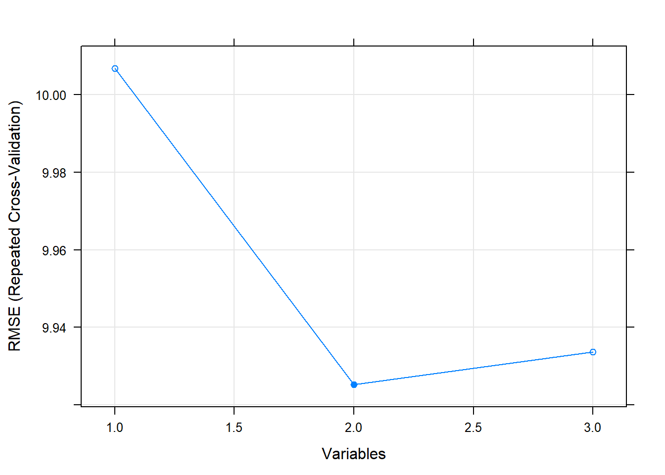
## [1] "group_x_drug" "group"##
## Call:
## lm(formula = y ~ ., data = tmp)
##
## Coefficients:
## (Intercept) group_x_drug group
## 50.501 9.698 3.296Think about the implications of these two sets of results for using any subsetting procedure to select interactions
Do you have concerns about an interaction if its lower order effects were available but not selected, as in this second example?
Would you have concerns if the lower order effects werent available to be selected? In other words, what if x_all only included the product term but not the dummy coded features for group and drug? This scenario was not displayed here but you might try it out yourself.
Caret also has a general univariate filtering technique for variable selection, \(sbf()\).
- For classification problems, it selects predictors using an ANOVA with the outcome as IV
- For regression, it uses a generalized additive model (GAM) and selections predictors if there is any functional relationship between the two
- After univariate filter, the selected predictors are then used with some specified statistical algorithm
- Like \(rfe()\), it uses an outer wrapper of resampling to get an independent evaluation of model performance that is not subject to selection bias