4 Cross Validation Methods
4.1 Unit Overview
- Validation (hold-out) set approach
- Leave one out cross validation
- K-fold cross validation
- Repeated K-fold cross validation
- Bootstrap for cross validation
- Grouped k-fold cross validation
- Pre-processing within Caret cross validation (tuning hyper-parameters)
- Cross validation approaches for simutaneous model selection and evaluation
We use cross validation for two goals:
- To select among model configurations
- To evaluate the performance of our models in new data
There are two kinds of problems that can emerge from selecting a suboptimal validation approach
- We can get a biased estimate of model performance (i.e., we can systematically under or over-estimate its performance)
- We can get an imprecise estimate of model performance (i.e., high variance in our model performance metric)
Essentially, this is the bias and variance problem again, but now not with respect to the model’s actual performance but instead with our estimate of how the model will perform
Lets get a dataset for this unit. We will use the heart disease dataset from the UCI Machine Learning Repository. We will focus on the Cleveland data subset.
NOTE:
- No spaces for factor levels (to avoid bad variable names with spaces or dots)
- Explicit assignment of dplyr::select to avoid conflict with \(select()\) in MASS
library(tidyverse)
library(caret)
library(rsample)
select <- dplyr::select

data_path <- "data"
d_all <- read_csv(file.path(data_path, "cleveland.csv"), col_names = FALSE, na = "?") %>%
  rename(age = X1,
         sex = X2,
         cp = X3,
         rest_bp = X4,
         chol = X5,
         fbs = X6,
         rest_ecg = X7,
         max_hr = X8,
         ex_ang = X9,
         ex_st_depress = X10,
         ex_st_slope = X11,
         ca = X12,
         thal = X13,
         disease = X14) %>%
  mutate(disease = factor(disease, levels = c(0:4), labels = c("no", "yes", "yes", "yes", "yes")),
         sex = factor(sex, levels = c(0,1), labels = c("female", "male")),
         cp = factor(cp, levels = c(1:4),
                     labels = c("typicalangina", "atypicalangina", "nonanginalpain", "nonanginalpain")),
         fbs = factor(fbs, levels = c(0,1), labels = c("False", "True")),
         rest_ecg = factor(rest_ecg, levels = c(0:2),  labels = c("normal", "sttwaveabnormality", "leftventricularhypertrophymax")),
         ex_ang = factor(ex_ang, levels = c(0,1), labels = c("no", "yes")),
         ex_st_slope = factor(ex_st_slope, levels = c(1:3), labels = c("upslope", "flat", "downslope")),
thal = factor(thal, levels = c(3,6,7), labels = c("normal", "fixeddefect", "reversabledefect")))- Coding Dummy variables directly (emerging as preferred processing pipeline for me in Caret)
- Removing missing data (for cleaner example)
- Removing nzv variable (for cleaner example)
dmy <- dummyVars(~ ., data = d_all, sep = "_", fullRank = TRUE)

d <- as_tibble(predict(dmy, d_all)) %>%
  select(-disease_yes) %>%
  mutate(disease = d_all$disease) %>%
  drop_na() %>%
  select(-rest_ecg_sttwaveabnormality) %>%
  glimpse()
## Observations: 297
## Variables: 17
## $ age <dbl> 63, 67, 67, 37, 41, 56, 62, 57, 63, 53, 5…
## $ sex_male <dbl> 1, 1, 1, 1, 0, 1, 0, 0, 1, 1, 1, 0, 1, 1,…
## $ cp_atypicalangina <dbl> 0, 0, 0, 0, 1, 1, 0, 0, 0, 0, 0, 1, 0, 1,…
## $ cp_nonanginalpain <dbl> 0, 1, 1, 1, 0, 0, 1, 1, 1, 1, 1, 0, 1, 0,…
## $ rest_bp <dbl> 145, 160, 120, 130, 130, 120, 140, 120, 1…
## $ chol <dbl> 233, 286, 229, 250, 204, 236, 268, 354, 2…
## $ fbs_True <dbl> 1, 0, 0, 0, 0, 0, 0, 0, 0, 1, 0, 0, 1, 0,…
## $ rest_ecg_leftventricularhypertrophymax <dbl> 1, 1, 1, 0, 1, 0, 1, 0, 1, 1, 0, 1, 1, 0,…
## $ max_hr <dbl> 150, 108, 129, 187, 172, 178, 160, 163, 1…
## $ ex_ang_yes <dbl> 0, 1, 1, 0, 0, 0, 0, 1, 0, 1, 0, 0, 1, 0,…
## $ ex_st_depress <dbl> 2.3, 1.5, 2.6, 3.5, 1.4, 0.8, 3.6, 0.6, 1…
## $ ex_st_slope_flat <dbl> 0, 1, 1, 0, 0, 0, 0, 0, 1, 0, 1, 1, 1, 0,…
## $ ex_st_slope_downslope <dbl> 1, 0, 0, 1, 0, 0, 1, 0, 0, 1, 0, 0, 0, 0,…
## $ ca <dbl> 0, 3, 2, 0, 0, 0, 2, 0, 1, 0, 0, 0, 1, 0,…
## $ thal_fixeddefect <dbl> 1, 0, 0, 0, 0, 0, 0, 0, 0, 0, 1, 0, 1, 0,…
## $ thal_reversabledefect <dbl> 0, 0, 1, 0, 0, 0, 0, 0, 1, 1, 0, 0, 0, 1,…
## $ disease <fct> no, yes, yes, no, no, no, yes, no, yes, y…We have:
- 297 cases
- 16 predictor variables including original numeric and dummy variables
- a dichotomous outcome (yes or no for heart disease) as a factor
4.2 The single validation (hold-out; test) set approach
To date, you have learned how to do the single validation set approach
With this approach, we would take our full n = 297 and:
- Split into one training and one test set
- Fit a model in our training set
- Use this trained model to predict scores in test
- Calculate accuracy (or some other metric) based on predicted and observed scores in test
- Report this performance metric from test as our estimate of the performance of our model in new data
What do you know about the performance of a model fit with n = 297 vs. a model fit in some subset (e.g., 80%, 50%) that we designate as a training set?
- The model fit in the subset of training data will perform less well than the model fit to the full n = 297. It will have more variance/be more overfit.
Given this, how can you train the best performing model in a study with n = 297?
- We should train the final model using the full n available to us. The training/test split is only used to estimate the performance of this final model.
If our true model is trained with n = 297, what can you say about our estimate of its performance using this single train/test split that only trains on a subset of the available data?
- Our performance estimate of our final model will be biased. Our performance estimate will likely underestimate the true performance of our final model trained with n = 297 because we are evaluating a trained model that will be more overfit than this model because it was trained with a smaller n.
Contrast the costs/benefits of a 50/50 vs. 80/20 split for train and test
- Using a training set with 80% of the sample will yield a less biased (under) estimate of the final (using all data) model performance than a training set with 50% of the sample. However, using a test set of 20% of the data will produce a more variable estimate of performance than the 50% test set. This is another bias-variance trade off but now instead of talking about model performance, we are seeing that we have to trade off bias and variance in our estimate of that the model performance too!
You have been doing the validation set approach all along but here is one final example with a 50/50 split
NOTES:
- Use of x and y rather than formula (another emerging preference for me. You get what you explicitly code into x)
- Conversion of x to data.frame
- Specification of positive level in \(confusionMatrix()\) (not necessary for accuracy)
set.seed(20140102)
splits <- initial_split(d, prop = .50, strata = "disease")
trn <- training(splits)
test <- testing(splits)

trn_x <- trn %>%
  select(-disease) %>%
  as.data.frame()

trn_y <- trn %>%
  pull(disease)

tc_no_cv <- trainControl(method = "none")
m_vs <- train(x = trn_x, y = trn_y,
              method = "glm", family = "binomial",
              trControl = tc_no_cv)

cm <- confusionMatrix(predict(m_vs, test), test$disease, positive = "yes")

cm
## Confusion Matrix and Statistics
##
## Reference
## Prediction no yes
## no 68 17
## yes 12 51
##
## Accuracy : 0.8041
## 95% CI : (0.7309, 0.8647)
## No Information Rate : 0.5405
## P-Value [Acc > NIR] : 1.858e-11
##
## Kappa : 0.6033
##
## Mcnemar's Test P-Value : 0.4576
##
## Sensitivity : 0.7500
## Specificity : 0.8500
## Pos Pred Value : 0.8095
## Neg Pred Value : 0.8000
## Prevalence : 0.4595
## Detection Rate : 0.3446
## Detection Prevalence : 0.4257
## Balanced Accuracy : 0.8000
##
## 'Positive' Class : yes
## There are multiple fields associated with the cm object. You can extract whichever you need
## [1] "positive" "table" "overall" "byClass" "mode" "dots"## [1] "Accuracy" "Kappa" "AccuracyLower" "AccuracyUpper" "AccuracyNull"
## [6] "AccuracyPValue" "McnemarPValue"## [1] 0.8040541Train a final model with the full n
#retrain final model with ALL data
all_x <- d %>%
  select(-disease) %>%
  as.data.frame()

all_y <- d %>%
  pull(disease)

m_final <- train(x = all_x, y = all_y,
                 method = "glm", family = "binomial",
                 trControl = tc_no_cv)
You will report an accuracy of .804 (last slide) as an estimate of the performance of your final model. However, the performance estimate using m_trn:
Will be a biased (under) estimate of the performance of the full model because the smaller n will lead it to be more overfit
Will have high variance (relative to other CV methods). If you formed many different test sets of n = 148, the performance of your m_trn model will vary widely across these different test sets (i.e., high standard error for the accuracy)
4.3 Leave One Out Cross Validation
How could you use this validation test set approach to get the least biased estimate of model performance with your n = 297 dataset that would still allow you to estimate its performance in a held out test set?
- Put all but one case into the training set (i.e., leave only one case out in the held out test set). In our example, you would train a model with n = 296. This model will have almost exactly the same problem with overfit as n = 297 so it will not yield much bias in estimating the performance of the n = 297 model.
What will be the biggest problem with this approach?
- You will estimate performance with only n = 1 in the test set. This means there will be high variance in your performance estimate.
How can you reduce this problem?
- Repeat this split between training and test n times so that there are n different sets of n=1 held out test sets. Then average the performance across all n of these test sets to get a more stable estimate of performance. This is Leave One Out Cross-validation.
Lets start doing some simple parallel processing on our local computer
Set up a parallel backend for Caret to use
Note that \(set.seed()\) may not be sufficient to produce reproducible results across multiple runs. Caret help provides alternative solutions. You can also read more on parallel processing in Caret or some discussion on Stack Overflow.
## [1] 8if(n_core > 2) {
cl <- makeCluster(n_core - 1, outfile = "")
registerDoParallel(cl)
getDoParWorkers()
}## [1] 7How will train implement LOOCV in parallel?
- Caret needs to train n models (each in a separate training set with n-1 observations) and then evaluate each of those models in the held out observation for that iteration. Each of these iterations are independent of each other and the order they are done doesnt matter. This is the perfect situation for parallel processing. You can have different CV iterations done at the same time across multiple cores on your machine and then aggregate these results at the end. train() will do this automatically for you.
Parallel Options
- Local using parallel training within Caret. \(allowParallel = TRUE\) is default for \(trainControl()\)
- Local using \(foreach()\) loop
- Split across multiple computers using condor and CHTC
An example of Leave One Out CV
NOTES:
- New train control object using LOOCV method
- Input full dataset for training and cv
- No need to split data using rsample - splits are handled by Caret
- Reproducible splits for Caret using \(set.seed()\)
- \(savePredictions\) and \(classProbs\) are useful in many instances
tc_loo <- trainControl(method = "LOOCV",
                       savePredictions = TRUE, classProbs = TRUE)

set.seed(20140102)
m_loo <- train(x = all_x, y = all_y,
               method = "glm", family = "binomial",
               trControl = tc_loo)

m_loo
## Generalized Linear Model
##
## 297 samples
## 16 predictor
## 2 classes: 'no', 'yes'
##
## No pre-processing
## Resampling: Leave-One-Out Cross-Validation
## Summary of sample sizes: 296, 296, 296, 296, 296, 296, ...
## Resampling results:
##
## Accuracy Kappa
## 0.8282828 0.6535849Lets look at resampling results
- Results contain only one row b/c there is only one model configuration (true for all situations where we only train a single model configuration)
- We can access predicted values using \(pred\) field of model object
- We can use the predicted values in test to calculate accuracy directly
##   parameter  Accuracy     Kappa
## 1 none 0.8282828 0.6535849## pred obs no yes rowIndex parameter
## 1 no no 0.913391373 0.08660863 1 none
## 2 yes yes 0.001720143 0.99827986 2 none
## 3 yes yes 0.005713812 0.99428619 3 none
## 4 no no 0.754451787 0.24554821 4 none
## 5 no no 0.964502654 0.03549735 5 none
## 6 no no 0.955958324 0.04404168 6 none
## 7 yes yes 0.341447394 0.65855261 7 none
## 8 no no 0.923763953 0.07623605 8 none
## 9 yes yes 0.086648509 0.91335149 9 none
## 10 yes yes 0.299519931 0.70048007 10 none
## 11 no no 0.638765885 0.36123412 11 none
## 12 no no 0.813916173 0.18608383 12 none
## 13 yes yes 0.242965666 0.75703433 13 none
## 14 no no 0.788306282 0.21169372 14 none
## 15 no no 0.717731716 0.28226828 15 none## [1] 0.8282828A final model is automatically fit to the full dataset and returned when using any CV method within Caret
This can be accessed within the \(finalModel\) field of the model object
##
## Call:
## NULL
##
## Deviance Residuals:
##     Min       1Q   Median       3Q      Max
## -3.0554  -0.5166  -0.1860   0.4209   2.6271
##
## Coefficients:
##                                         Estimate Std. Error z value Pr(>|z|)
## (Intercept)                            -4.887967   2.815615  -1.736 0.082560 .
## age                                    -0.017689   0.023674  -0.747 0.454954
## sex_male                                1.377612   0.491448   2.803 0.005060 **
## cp_atypicalangina                       1.139527   0.760405   1.499 0.133983
## cp_nonanginalpain                       1.218939   0.606795   2.009 0.044557 *
## rest_bp                                 0.024572   0.010914   2.251 0.024365 *
## chol                                    0.004064   0.003780   1.075 0.282314
## fbs_True                               -1.043996   0.545892  -1.912 0.055817 .
## rest_ecg_leftventricularhypertrophymax  0.465793   0.368019   1.266 0.205629
## max_hr                                 -0.021727   0.010477  -2.074 0.038102 *
## ex_ang_yes                              1.128382   0.405456   2.783 0.005386 **
## ex_st_depress                           0.282296   0.212903   1.326 0.184861
## ex_st_slope_flat                        1.048519   0.449672   2.332 0.019714 *
## ex_st_slope_downslope                   0.489670   0.821231   0.596 0.550999
## ca                                      1.342950   0.266018   5.048 4.46e-07 ***
## thal_fixeddefect                        0.338307   0.757214   0.447 0.655035
## thal_reversabledefect                   1.499955   0.404951   3.704 0.000212 ***
## ---
## Signif. codes:  0 '***' 0.001 '**' 0.01 '*' 0.05 '.' 0.1 ' ' 1
##
## (Dispersion parameter for binomial family taken to be 1)
##
##     Null deviance: 409.95  on 296  degrees of freedom
## Residual deviance: 206.63  on 280  degrees of freedom
## AIC: 240.63
##
## Number of Fisher Scoring iterations: 6
Comparisons across LOOCV and Single Validation set
The performance estimate from LOOCV has less bias than the validation set method (because the models that are evaluated were fit with close to the full n of the final model)
LOOCV uses all observations as “test” at some point. Less variance than single 20% or 50% test set?
LOOCV is not “random” - only one solution given a dataset. People note this as an advantage but I dont think this really matters…..
But…
- LOOCV can be computationally expensive (need to fit and evaluate n models)
LOOCV uses all the data in test across the ‘n’ test sets. Averaging also helps reduce variance in the performance metric.
However, averaging reduces variance to a greater degree when the performance measures being averaged are less related/more independent.
The n models are VERY similar in LOOCV b/c they are each trained on almost the same data (each have n-1 observations)
K-fold cross validation improves the variance of the average performance metric by averaging across more independent training sets
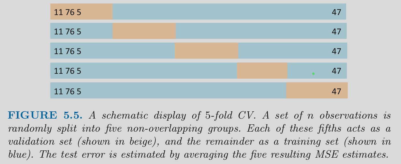
4.4 K-fold Cross Validation
K-fold cross validation
- Divide the observations into K equal size independent “folds” (each observation appears in only one fold)
- Hold out 1 of these folds (1/Kth of the dataset) to use as a test set
- Fit/train a model in the remaining K-1 folds
- Repeat until each of the folds has been held out once
- Performance estimate is the average performance across the K held out folds
Common values of K are 5 and 10
NOTES:
K-fold fit and evaluated K different models
Performance estimate is average of these models
It is estimate of performance of any model trained with the n associated with K-1 folds, the statistical algorithm (and its hyperparameters), and the feature/predictor set
- Bias exists when the n of trained models is very different from the full n
- Variance is a function of how performance estimate is derived (n of test, averaging of estimates, correlations among averaged models)
This is true for all single loop (vs. nested) CV approaches
Visualization of K-fold
An example of K-fold Cross-validation
NOTES:
- New train control object using cv and number (k)
- Input full dataset for training and cv
- No need to split data using rsample - splits are handled by Caret
- Reproducible splits for Caret using \(set.seed()\)
- Saving individual predictions in test (if you want them) for the K held out test sets
- Class probabilities are also useful for other thresholds (true for any of these methods but demo here)
tc_kfold <- trainControl(method = "cv", number = 10,
                         savePredictions = TRUE, classProbs = TRUE)

set.seed(20140102)
m_kfold <- train(x = all_x, y = all_y,
                 method = "glm", family = "binomial",
                 trControl = tc_kfold)

m_kfold
## Generalized Linear Model
##
## 297 samples
## 16 predictor
## 2 classes: 'no', 'yes'
##
## No pre-processing
## Resampling: Cross-Validated (10 fold)
## Summary of sample sizes: 268, 267, 268, 267, 267, 267, ...
## Resampling results:
##
## Accuracy Kappa
## 0.822069 0.6408114Lets look at resampling results
- You can access predictions within \(pred\) as before
- You could calculate accuracy for any specific held-out test set using \(pred\) and \(obs\) subfields of \(pred\)
- Could plot ROC curve using the probabilities that we choose to save here (or more accurately the K curves for each trained model)
##   parameter Accuracy     Kappa AccuracySD   KappaSD
## 1 none 0.822069 0.6408114 0.0643126 0.1310542## pred obs no yes rowIndex parameter Resample
## 1 no no 0.96630081 0.03369919 5 none Fold01
## 2 yes yes 0.04674286 0.95325714 30 none Fold01
## 3 no yes 0.91119604 0.08880396 33 none Fold01
## 4 no no 0.55851346 0.44148654 42 none Fold01
## 5 no yes 0.73252566 0.26747434 58 none Fold01## pred obs no yes rowIndex parameter Resample
## 293 no no 0.6002613 0.39973868 231 none Fold10
## 294 no no 0.9821942 0.01780578 240 none Fold10
## 295 no no 0.9372655 0.06273449 276 none Fold10
## 296 no yes 0.6923029 0.30769705 288 none Fold10
## 297 no yes 0.9047138 0.09528620 290 none Fold10## pred obs no yes rowIndex parameter Resample
## 1 no no 0.966300814 0.03369919 5 none Fold01
## 2 yes yes 0.046742858 0.95325714 30 none Fold01
## 3 no yes 0.911196040 0.08880396 33 none Fold01
## 4 no no 0.558513462 0.44148654 42 none Fold01
## 5 no yes 0.732525660 0.26747434 58 none Fold01
## 6 yes no 0.267207203 0.73279280 60 none Fold01
## 7 no no 0.871944183 0.12805582 83 none Fold01
## 8 no no 0.944705524 0.05529448 85 none Fold01
## 9 no no 0.849997241 0.15000276 87 none Fold01
## 10 yes yes 0.006689340 0.99331066 91 none Fold01
## 11 yes yes 0.205714034 0.79428597 106 none Fold01
## 12 no no 0.957393943 0.04260606 112 none Fold01
## 13 yes yes 0.003873930 0.99612607 118 none Fold01
## 14 yes no 0.227720407 0.77227959 144 none Fold01
## 15 yes no 0.095888984 0.90411102 175 none Fold01
## 16 yes yes 0.425278793 0.57472121 179 none Fold01
## 17 no no 0.808049337 0.19195066 202 none Fold01
## 18 yes yes 0.002365706 0.99763429 204 none Fold01
## 19 no no 0.951743314 0.04825669 228 none Fold01
## 20 no no 0.953421348 0.04657865 236 none Fold01
## 21 no no 0.972973537 0.02702646 253 none Fold01
## 22 no no 0.819693828 0.18030617 254 none Fold01
## 23 no no 0.903658009 0.09634199 255 none Fold01
## 24 no no 0.852421447 0.14757855 256 none Fold01
## 25 yes yes 0.438449513 0.56155049 281 none Fold01
## 26 yes yes 0.057229919 0.94277008 283 none Fold01
## 27 yes yes 0.033191247 0.96680875 292 none Fold01
## 28 yes yes 0.029105940 0.97089406 296 none Fold01
## 29 no yes 0.867668403 0.13233160 297 none Fold01## [1] 0.7931034We can also look at the (small) sampling distribution for accuracy for a single K-fold performance estimate from one held-out test set
You can report SD of the performance estimates to understand the standard error of your performance metric
folds <- m_kfold$pred %>%
  group_by(Resample) %>%
  summarise(accuracy = mean(pred == obs)) %>%
  glimpse()
## Observations: 10
## Variables: 2
## $ Resample <chr> "Fold01", "Fold02", "Fold03", "Fold04", "Fold05", "Fold06", "Fold07", "…
## $ accuracy <dbl> 0.7931034, 0.8333333, 0.8965517, 0.7333333, 0.8333333, 0.8000000, 0.866…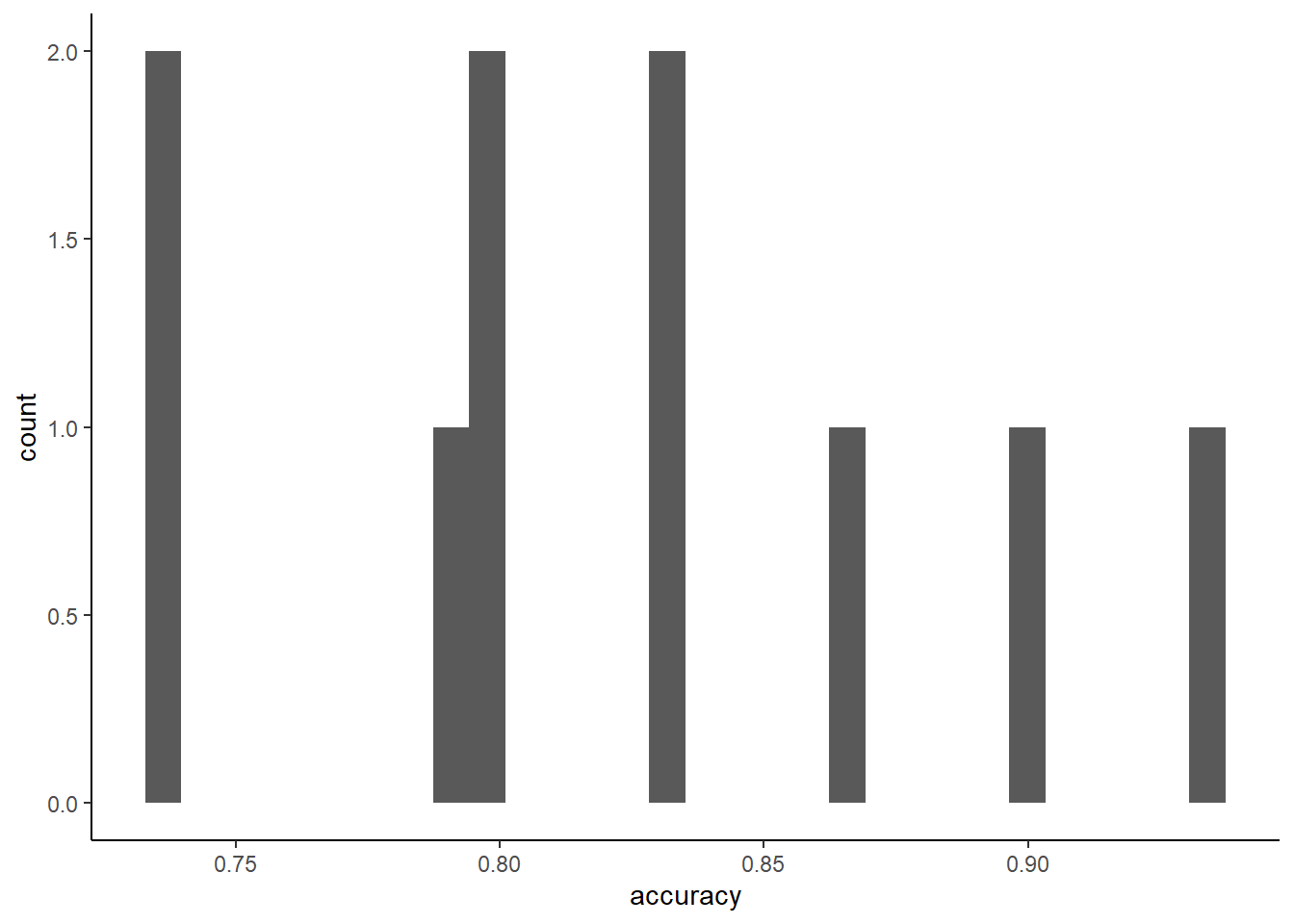
## [1] 0.0643126You can use the probabilities with a different threshold (not .5) to get different class predictions that have different sensitivity and specificity (but lower overall accuracy)
m_kfold$pred %>%
  mutate(pred_25 = if_else(yes > .25, "yes", "no")) %>%
  group_by(Resample) %>%
  summarise(accuracy = mean(pred_25 == obs)) %>%   #accuracy for each of 10 folds
  print(10) %>%
  summarise (mean(accuracy))  #mean accuracy across 10 folds
## # A tibble: 10 x 2
## Resample accuracy
## <chr> <dbl>
## 1 Fold01 0.793
## 2 Fold02 0.8
## 3 Fold03 0.931
## 4 Fold04 0.633
## 5 Fold05 0.867
## 6 Fold06 0.833
## 7 Fold07 0.833
## 8 Fold08 0.767
## 9 Fold09 0.828
## 10 Fold10 0.667## # A tibble: 1 x 1
## `mean(accuracy)`
## <dbl>
## 1 0.795Comparisons between K-fold vs. LOOCV and Single Validation set
For Bias
- K-fold typically has less bias than the validation set method
- E.g. 10-fold trains models with 9/10th of the data vs. 50% or 80%, etc
- K Fold has somewhat more bias than LOOCV because LOOCV uses n-1 observations for training/fitting models
For Variance
K-fold has less variance than LOOCV
- Like LOOCV, it uses all observations in test at some point
- The averaged models are more independent b/c models are trained on less overlapping datasets
K-fold has less variance than validation set b/c uses all data and averages
K-fold is less computationally expensive than LOOCV (though more expensive than single validation set)
K-fold is still “random” (but so what?)
K-fold is generally preferred over both of these other approaches
- But exploration?
4.5 Repeated K-fold Cross Validation
You can repeat the K-fold procedure multiple times with new splits for a different mix of K folds
Two benefits:
- More stable performance estimate (because averaged over more folds: repeats * K)
- Many more estimates of performance to characterize (SD; plot) of your performance estimate
But it is computationally expensive (depending on number of repeats)
An example of Repeated K-fold Cross-validation
NOTES:
- New train control object using repeatedcv, number (k), and repeats
- Input full dataset for training and cv
- No need to split data using rsample - splits are handled by Caret
- Reproducible splits for Caret using \(set.seed()\)
- Saving predictions and probabilities
tc_rep_kfold <- trainControl(method = "repeatedcv", number = 10, repeats = 10,
                             savePredictions = TRUE, classProbs = TRUE)

set.seed(20140102)
m_rep_kfold <- train(x = all_x, y = all_y,
                     method = "glm", family = "binomial",
                     trControl = tc_rep_kfold)

m_rep_kfold
## Generalized Linear Model
##
## 297 samples
## 16 predictor
## 2 classes: 'no', 'yes'
##
## No pre-processing
## Resampling: Cross-Validated (10 fold, repeated 10 times)
## Summary of sample sizes: 268, 267, 268, 267, 267, 267, ...
## Resampling results:
##
## Accuracy Kappa
## 0.8206092 0.637837Lets look at resampling results
##   parameter  Accuracy    Kappa AccuracySD   KappaSD
## 1 none 0.8206092 0.637837 0.06545524 0.1323482## pred obs no yes rowIndex parameter Resample
## 1 no no 0.96630081 0.03369919 5 none Fold01.Rep01
## 2 yes yes 0.04674286 0.95325714 30 none Fold01.Rep01
## 3 no yes 0.91119604 0.08880396 33 none Fold01.Rep01
## 4 no no 0.55851346 0.44148654 42 none Fold01.Rep01
## 5 no yes 0.73252566 0.26747434 58 none Fold01.Rep01
## 6 yes no 0.26720720 0.73279280 60 none Fold01.Rep01
## 7 no no 0.87194418 0.12805582 83 none Fold01.Rep01
## 8 no no 0.94470552 0.05529448 85 none Fold01.Rep01
## 9 no no 0.84999724 0.15000276 87 none Fold01.Rep01
## 10 yes yes 0.00668934 0.99331066 91 none Fold01.Rep01## pred obs no yes rowIndex parameter Resample
## 2961 no no 0.98509942 0.01490058 208 none Fold10.Rep10
## 2962 no no 0.62505162 0.37494838 210 none Fold10.Rep10
## 2963 no no 0.94229283 0.05770717 228 none Fold10.Rep10
## 2964 yes yes 0.01060943 0.98939057 233 none Fold10.Rep10
## 2965 no no 0.92292429 0.07707571 274 none Fold10.Rep10
## 2966 no yes 0.70925568 0.29074432 275 none Fold10.Rep10
## 2967 yes yes 0.12449611 0.87550389 279 none Fold10.Rep10
## 2968 no no 0.94634275 0.05365725 285 none Fold10.Rep10
## 2969 no no 0.97503293 0.02496707 291 none Fold10.Rep10
## 2970 no yes 0.88342539 0.11657461 297 none Fold10.Rep10Lets look at sampling distribution for a single K-fold performance estimate
Could also report the standard deviation (standard error) for our accuracy estimate
repeats <- m_rep_kfold$pred %>%
  group_by(Resample) %>%
  summarise(accuracy = mean(pred == obs))

ggplot(data = repeats, aes(x = accuracy)) +
  geom_histogram(bins = 12)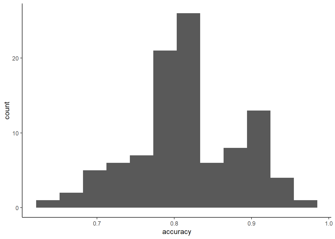
## [1] 0.06545524Comparisons between repeated K-fold and K-fold
Repeated K-fold:
- Has same bias as K-fold
- Has all the benefits of single K-fold
- Has even more stable estimate of performance (mean over more folds/repeats)
- Provides more info about distribution for the performance estimate
- But is more computationally expensive
Repeated K-fold is preferred over K-fold to the degree possible based on computational limitations (parallel, N, p, statistical algorithm, # of model configurations)
4.6 Bootstrapping for Cross Validation
A bootstrap sample is a random sample taken with replacement (i.e., same observations can be sampled multiple times within one bootstrap sample)
If you bootstrap a new sample of size n from a dataset with sample size n, approximately 63.2% of the original observations end up in the bootstrap sample
The remaining 36.8% of the observations are called the “out of bag” samples
Bootstrapping for cross validation:
- Creates B bootstrap samples of size n = n from the original dataset
- For any specific bootstrap (b)
- Model(s) are fit to the bootstrap sample
- Model performance is evaluated in the associated out of bag (held-out) samples
- This is repeated B times such that you have B assessments of model performance
An example of Bootstrapping for Cross-validation
NOTES:
- New train control object using boot and number
- Input full dataset for training and cv
- No need to split data using rsample - splits are handled by Caret
- Reproducible splits for Caret using \(set.seed()\)
- Saving prediction and probabilities
tc_boot <- trainControl(method = "boot", number = 100,
                        savePredictions = TRUE, classProbs = TRUE)

set.seed(20140102)
m_boot <- train(x = all_x, y = all_y,
                method = "glm", family = "binomial",
                trControl = tc_boot)

m_boot
## Generalized Linear Model
##
## 297 samples
## 16 predictor
## 2 classes: 'no', 'yes'
##
## No pre-processing
## Resampling: Bootstrapped (100 reps)
## Summary of sample sizes: 297, 297, 297, 297, 297, 297, ...
## Resampling results:
##
## Accuracy Kappa
## 0.8154762 0.627255Lets look at resampling results from Bootstrapping CV
##   parameter  Accuracy    Kappa AccuracySD    KappaSD
## 1 none 0.8154762 0.627255 0.03490279 0.07056302## pred obs no yes rowIndex parameter Resample
## 1 no no 9.696081e-01 0.030391904 1 none Resample001
## 2 yes yes 6.103692e-05 0.999938963 2 none Resample001
## 3 yes yes 1.803654e-03 0.998196346 3 none Resample001
## 4 no no 9.768248e-01 0.023175209 5 none Resample001
## 5 no yes 7.720910e-01 0.227909025 10 none Resample001
## 6 yes yes 9.400669e-02 0.905993307 13 none Resample001
## 7 no no 8.533729e-01 0.146627078 14 none Resample001
## 8 no yes 9.402185e-01 0.059781546 17 none Resample001
## 9 no no 9.255276e-01 0.074472373 20 none Resample001
## 10 no no 9.980985e-01 0.001901535 22 none Resample001## pred obs no yes rowIndex parameter Resample
## 10897 no no 0.955306568 0.04469343 253 none Resample100
## 10898 no no 0.921389371 0.07861063 254 none Resample100
## 10899 no yes 0.905773715 0.09422629 259 none Resample100
## 10900 no no 0.904620889 0.09537911 261 none Resample100
## 10901 yes yes 0.123204568 0.87679543 262 none Resample100
## 10902 yes yes 0.080329591 0.91967041 267 none Resample100
## 10903 yes yes 0.002461687 0.99753831 269 none Resample100
## 10904 no no 0.877920322 0.12207968 278 none Resample100
## 10905 yes yes 0.207188776 0.79281122 286 none Resample100
## 10906 yes yes 0.100820991 0.89917901 295 none Resample100##
## Resample001 Resample002 Resample003 Resample004 Resample005 Resample006 Resample007
## 116 117 113 110 112 108 112
## Resample008 Resample009 Resample010
## 105 112 99Lets look at sampling distribution for a single bootstrap resample
Could also report SD of held-out folds accuracy across bootstraps
boots <- m_boot$pred %>%
  group_by(Resample) %>%
  summarise(accuracy = mean(pred == obs))

ggplot(data = boots, aes(x = accuracy)) +
  geom_histogram(bins = 12)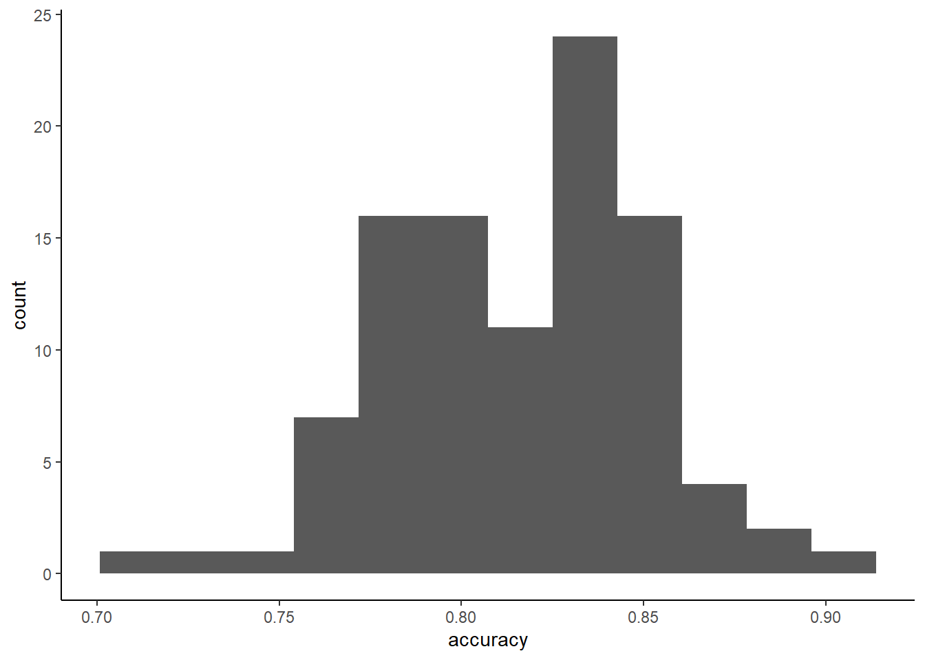
## [1] 0.03490279Relevant comparisons, strengths/weaknesses for bootstrap for CV
Higher bias than k-fold using typical k values (bias equivalent to about k = 2)
- Although training sets have full n, they only include about 63% unique observations. These models under perform training sets with 80 - 90% unique observations
- With smaller training set sizes, this bias is considered too high by some (Kuhn)
Has less variance than K-fold
- With 1000 bootstraps (and test sets with ~ 37% of n) can get a very precise estimate of test error
Can also represent the variance of our test error (like repeated K-fold)
Used primarily for selecting among model configurations when you don’t care about bias and just want precise selection metric
- Useful in explanation scenarios where you just need the “best” model
- “Inner loop” of nested cross validation (more on this later)
4.7 Grouped K-fold
How should you generally handle situations where you have repeated observations from the same participant? What is the concern?
- You can often predict an individuals own data better using some of their own data. If your model will not ever encounter that individual again, this will bias your estimate of your models performance. You can remove that bias by making sure that all observations from an individual are grouped together so that they always end up in either train or test but never both. Easy to do a grouped K-fold or grouped single validation set approach. Not too hard to write code to adjust other approaches (LOOCV, Bootstrap) it for other approaches but probably not needed b/c K-fold (and repeated K-fold) are generally good CV techniques.
Caret doesnt directly support grouped resampling but \(rsample\) package does
Lets do a simple example of grouped K-fold on simulated data
Make a data set with 100 unique participants & 10 observations of x and y for each participant
x & y are correlated around .33
then median split Y to make it a classification problem (as our other examples)
d_grouped <- tibble(ID = rep(1:100, each = 10),
                    x = rnorm(length(ID)),
                    y = rnorm(length(x), x, 3)) %>%
  mutate(y = if_else(y < median(y),0,1),
         y = factor(y, levels = c(0,1), labels = c("low", "high")))

print(d_grouped, n = 25)
## # A tibble: 1,000 x 3
## ID x y
## <int> <dbl> <fct>
## 1 1 -1.32 low
## 2 1 0.623 high
## 3 1 -0.245 low
## 4 1 -0.106 high
## 5 1 0.777 high
## 6 1 0.635 high
## 7 1 0.852 low
## 8 1 0.158 high
## 9 1 0.189 low
## 10 1 -1.24 low
## 11 2 0.0765 high
## 12 2 -1.35 low
## 13 2 -1.68 low
## 14 2 -1.23 low
## 15 2 -0.0481 high
## 16 2 -0.232 high
## 17 2 2.33 low
## 18 2 -0.647 low
## 19 2 -2.53 low
## 20 2 0.0386 low
## 21 3 1.45 high
## 22 3 0.597 high
## 23 3 -0.0809 high
## 24 3 0.759 low
## 25 3 0.0589 high
## # … with 975 more rows- Use \(group\_vfold\_cv()\) to make grouped splits
- Specify the grouping variable (e.g, “ID”) and number of folds (v)
- The object that is returned cant be directly used by Caret’s \(train()\)
- However, \(rsample2caret()\) reformats it for use in Caret
- \(train()\) allow us to list row numbers for held-in (index) and held-out (indexOut) sets for multiple iterations
- \(rsample2caret()\) gives us these row numbers
set.seed(20140102)
splits <- group_vfold_cv(d_grouped, group = "ID", v = 10)

Caret_splits <- rsample2caret(splits)

names(Caret_splits)
## [1] "index" "indexOut"All observations for a participant are now either held-in (training) or held-out (test) in the index and indexOut lists
For example, lets look at the first set of held-in and held-out row numbers
- indexOut are our held-out samples. You can see we have all data from 10 participants (10 groups of 10 row numbers)
- index lists our held-in samples from this first resample. It does not include these row numbers (e.g, 41-50, 181-190, …)
##   [1]  31  32  33  34  35  36  37  38  39  40 181 182 183 184 185 186 187 188 189 190 241
##  [22] 242 243 244 245 246 247 248 249 250 431 432 433 434 435 436 437 438 439 440 481 482
##  [43] 483 484 485 486 487 488 489 490 761 762 763 764 765 766 767 768 769 770 811 812 813
##  [64] 814 815 816 817 818 819 820 831 832 833 834 835 836 837 838 839 840 911 912 913 914
## [85] 915 916 917 918 919 920 961 962 963 964 965 966 967 968 969 970## [1] 1 2 3 4 5 6 7 8 9 10 11 12 13 14 15 16 17
## [18] 18 19 20 21 22 23 24 25 26 27 28 29 30 41 42 43 44
## [35] 45 46 47 48 49 50 51 52 53 54 55 56 57 58 59 60 61
## [52] 62 63 64 65 66 67 68 69 70 71 72 73 74 75 76 77 78
## [69] 79 80 81 82 83 84 85 86 87 88 89 90 91 92 93 94 95
## [86] 96 97 98 99 100 101 102 103 104 105 106 107 108 109 110 111 112
## [103] 113 114 115 116 117 118 119 120 121 122 123 124 125 126 127 128 129
## [120] 130 131 132 133 134 135 136 137 138 139 140 141 142 143 144 145 146
## [137] 147 148 149 150 151 152 153 154 155 156 157 158 159 160 161 162 163
## [154] 164 165 166 167 168 169 170 171 172 173 174 175 176 177 178 179 180
## [171] 191 192 193 194 195 196 197 198 199 200 201 202 203 204 205 206 207
## [188] 208 209 210 211 212 213 214 215 216 217 218 219 220 221 222 223 224
## [205] 225 226 227 228 229 230 231 232 233 234 235 236 237 238 239 240 251
## [222] 252 253 254 255 256 257 258 259 260 261 262 263 264 265 266 267 268
## [239] 269 270 271 272 273 274 275 276 277 278 279 280 281 282 283 284 285
## [256] 286 287 288 289 290 291 292 293 294 295 296 297 298 299 300 301 302
## [273] 303 304 305 306 307 308 309 310 311 312 313 314 315 316 317 318 319
## [290] 320 321 322 323 324 325 326 327 328 329 330 331 332 333 334 335 336
## [307] 337 338 339 340 341 342 343 344 345 346 347 348 349 350 351 352 353
## [324] 354 355 356 357 358 359 360 361 362 363 364 365 366 367 368 369 370
## [341] 371 372 373 374 375 376 377 378 379 380 381 382 383 384 385 386 387
## [358] 388 389 390 391 392 393 394 395 396 397 398 399 400 401 402 403 404
## [375] 405 406 407 408 409 410 411 412 413 414 415 416 417 418 419 420 421
## [392] 422 423 424 425 426 427 428 429 430 441 442 443 444 445 446 447 448
## [409] 449 450 451 452 453 454 455 456 457 458 459 460 461 462 463 464 465
## [426] 466 467 468 469 470 471 472 473 474 475 476 477 478 479 480 491 492
## [443] 493 494 495 496 497 498 499 500 501 502 503 504 505 506 507 508 509
## [460] 510 511 512 513 514 515 516 517 518 519 520 521 522 523 524 525 526
## [477] 527 528 529 530 531 532 533 534 535 536 537 538 539 540 541 542 543
## [494] 544 545 546 547 548 549 550 551 552 553 554 555 556 557 558 559 560
## [511] 561 562 563 564 565 566 567 568 569 570 571 572 573 574 575 576 577
## [528] 578 579 580 581 582 583 584 585 586 587 588 589 590 591 592 593 594
## [545] 595 596 597 598 599 600 601 602 603 604 605 606 607 608 609 610 611
## [562] 612 613 614 615 616 617 618 619 620 621 622 623 624 625 626 627 628
## [579] 629 630 631 632 633 634 635 636 637 638 639 640 641 642 643 644 645
## [596] 646 647 648 649 650 651 652 653 654 655 656 657 658 659 660 661 662
## [613] 663 664 665 666 667 668 669 670 671 672 673 674 675 676 677 678 679
## [630] 680 681 682 683 684 685 686 687 688 689 690 691 692 693 694 695 696
## [647] 697 698 699 700 701 702 703 704 705 706 707 708 709 710 711 712 713
## [664] 714 715 716 717 718 719 720 721 722 723 724 725 726 727 728 729 730
## [681] 731 732 733 734 735 736 737 738 739 740 741 742 743 744 745 746 747
## [698] 748 749 750 751 752 753 754 755 756 757 758 759 760 771 772 773 774
## [715] 775 776 777 778 779 780 781 782 783 784 785 786 787 788 789 790 791
## [732] 792 793 794 795 796 797 798 799 800 801 802 803 804 805 806 807 808
## [749] 809 810 821 822 823 824 825 826 827 828 829 830 841 842 843 844 845
## [766] 846 847 848 849 850 851 852 853 854 855 856 857 858 859 860 861 862
## [783] 863 864 865 866 867 868 869 870 871 872 873 874 875 876 877 878 879
## [800] 880 881 882 883 884 885 886 887 888 889 890 891 892 893 894 895 896
## [817] 897 898 899 900 901 902 903 904 905 906 907 908 909 910 921 922 923
## [834] 924 925 926 927 928 929 930 931 932 933 934 935 936 937 938 939 940
## [851] 941 942 943 944 945 946 947 948 949 950 951 952 953 954 955 956 957
## [868] 958 959 960 971 972 973 974 975 976 977 978 979 980 981 982 983 984
## [885] 985 986 987 988 989 990 991 992 993 994 995 996 997 998 999 1000Now lets use these grouped K-fold resamples in Caret
NOTE: use of \(index\) and \(indexOut\) arguments in \(trainControl()\)
tc_grouped <- trainControl(method = "cv", number = 10,
                           savePredictions = TRUE, classProbs = TRUE,
                           index = Caret_splits$index,
                           indexOut = Caret_splits$indexOut)

all_x <- d_grouped %>%
  select(-ID, -y) %>%
  as.data.frame()

all_y <- d_grouped %>%
  pull(y)

m_grouped <- train(x = all_x, y = all_y,
                   method = "glm", family = "binomial",
                   trControl = tc_grouped)

m_grouped
## Generalized Linear Model
##
## 1000 samples
## 1 predictor
## 2 classes: 'low', 'high'
##
## No pre-processing
## Resampling: Cross-Validated (10 fold)
## Summary of sample sizes: 900, 900, 900, 900, 900, 900, ...
## Resampling results:
##
## Accuracy Kappa
## 0.609 0.2167234.8 Using CV to Select Best Model Configurations
In all of the previous examples, we have used various cross-validation methods only to evaluate model performance in new data
CV is also used to select best models. Best means the model that performs the best in new data and therefore is closest to the true DGP for the data
One common scenario where you will do model selection is when “tuning” (picking) the appropriate hyperparameters for a statistical model (e.g., k in KNN). Caret help provides substantial information about hyperparameter tuning via cross validation. Strongly suggested reading.
You can also select among model configurations in an explanatory scenario to have a principled approach to determine the model configuration that best matches the true DGP (and would be best to test your hypotheses; e.g., selecting covariates, deciding on X transformations, outlier identification approach)
Lets use K-fold cross validation to select the best k for knn applied to our heart disease dataset (thats a lot of Ks!)
all_x <- d %>%
  select(-disease) %>%
  as.data.frame()

all_y <- d %>%
  pull(disease)

tc_kfold <- trainControl(method = "cv", number = 10,
                         savePredictions = TRUE, classProbs = TRUE)

set.seed(20140102)
m_kfold_knn <- train(x = all_x, y = all_y,
                     method = "knn",
                     trControl = tc_kfold)

m_kfold_knn
## k-Nearest Neighbors
##
## 297 samples
## 16 predictor
## 2 classes: 'no', 'yes'
##
## No pre-processing
## Resampling: Cross-Validated (10 fold)
## Summary of sample sizes: 268, 267, 268, 267, 267, 267, ...
## Resampling results across tuning parameters:
##
## k Accuracy Kappa
## 5 0.6497701 0.2883933
## 7 0.6629885 0.3174775
## 9 0.6397701 0.2704719
##
## Accuracy was used to select the optimal model using the largest value.
## The final value used for the model was k = 7.- Caret defaulted to evaluate 3 values of k for knn
- k = 9 provides the best bias-variance trade-off among these three values
You can access the results for all hyperparameters directly
##   k  Accuracy     Kappa AccuracySD   KappaSD
## 1 5 0.6497701 0.2883933 0.10130757 0.2104765
## 2 7 0.6629885 0.3174775 0.09283075 0.1894453
## 3 9 0.6397701 0.2704719 0.08287242 0.1674558
Caret also automatically trains a final model for you using the best tuning value for the hyperparameter with all of the observations (default; see \(indexFinal\) in \(trainControl()\))
##   k
## 2 7## 7-nearest neighbor model
## Training set outcome distribution:
##
## no yes
## 160 137You can use this best model automatically in \(predict()\)
Here are predictions back into the full dataset
##   [1] no  yes yes no  no  no  no  no  yes no  yes no  yes no  no  no  yes no  yes no  no
##  [22] no  no  no  yes no  no  yes no  yes no  yes yes no  no  no  yes yes yes no  yes no
##  [43] yes no  no  yes yes yes no  no  no  yes no  no  yes yes no  no  no  yes yes no  yes
##  [64] no  yes no  yes no  yes no  yes yes yes no  no  no  yes yes no  yes no  yes no  yes
##  [85] no  no  no  no  no  no  yes no  no  no  no  yes yes no  no  no  no  no  yes no  no
## [106] no  no  yes no  yes yes no  yes yes yes no  no  yes yes no  no  no  yes no  no  yes
## [127] yes no  no  yes no  no  no  no  no  yes yes yes no  no  yes no  yes yes no  yes no
## [148] no  no  yes yes no  yes yes yes no  no  yes yes no  yes no  yes no  no  no  no  yes
## [169] yes yes no  no  yes yes yes yes no  no  no  no  no  yes yes no  no  no  yes yes no
## [190] yes yes yes yes no  no  no  yes no  yes no  yes no  yes yes yes no  no  no  no  no
## [211] yes yes no  no  no  yes no  no  no  no  yes no  no  no  no  yes no  no  yes yes yes
## [232] no  yes yes yes no  no  no  no  no  no  yes yes yes yes no  yes yes yes yes no  no
## [253] no  no  yes no  yes no  yes no  no  yes yes yes no  no  yes no  yes no  no  yes no
## [274] no  no  yes yes no  yes no  yes yes yes no  no  yes no  no  yes yes no  yes yes yes
## [295] yes yes no
## Levels: no yes
You likely want to evaluate more than 3 values of k
Caret will automatically select more good choices for you
See \(tuneLength\) argument in \(train()\)
tc_kfold <- trainControl(method = "cv", number = 10,
                         savePredictions = TRUE, classProbs = TRUE)

set.seed(20140102)
m_kfold_knn50 <- train(x = all_x, y = all_y,
                       method = "knn",
                       trControl = tc_kfold,
                       tuneLength = 50)

m_kfold_knn50
## k-Nearest Neighbors
##
## 297 samples
## 16 predictor
## 2 classes: 'no', 'yes'
##
## No pre-processing
## Resampling: Cross-Validated (10 fold)
## Summary of sample sizes: 268, 267, 268, 267, 267, 267, ...
## Resampling results across tuning parameters:
##
## k Accuracy Kappa
## 5 0.6531034 0.2946870
## 7 0.6629885 0.3174775
## 9 0.6397701 0.2704719
## 11 0.6462069 0.2847430
## 13 0.6565517 0.3042528
## 15 0.6429885 0.2782284
## 17 0.6529885 0.2967799
## 19 0.6563218 0.3033552
## 21 0.6731034 0.3396912
## 23 0.6767816 0.3456311
## 25 0.6934483 0.3776990
## 27 0.6833333 0.3587564
## 29 0.6734483 0.3372818
## 31 0.6596552 0.3059844
## 33 0.6595402 0.3063698
## 35 0.6598851 0.3073338
## 37 0.6429885 0.2735483
## 39 0.6325287 0.2493264
## 41 0.6158621 0.2134469
## 43 0.6191954 0.2192097
## 45 0.6326437 0.2469868
## 47 0.6493103 0.2810765
## 49 0.6427586 0.2680136
## 51 0.6191954 0.2196535
## 53 0.6224138 0.2246722
## 55 0.6425287 0.2652431
## 57 0.6390805 0.2569110
## 59 0.6427586 0.2643655
## 61 0.6395402 0.2596664
## 63 0.6360920 0.2516933
## 65 0.6393103 0.2557566
## 67 0.6258621 0.2262618
## 69 0.6359770 0.2480220
## 71 0.6459770 0.2686925
## 73 0.6495402 0.2755113
## 75 0.6462069 0.2681505
## 77 0.6327586 0.2406470
## 79 0.6428736 0.2604854
## 81 0.6427586 0.2599318
## 83 0.6494253 0.2737088
## 85 0.6497701 0.2742781
## 87 0.6429885 0.2608585
## 89 0.6498851 0.2750210
## 91 0.6465517 0.2678604
## 93 0.6363218 0.2471627
## 95 0.6363218 0.2465400
## 97 0.6294253 0.2327520
## 99 0.6396552 0.2536947
## 101 0.6295402 0.2324664
## 103 0.6294253 0.2315603
##
## Accuracy was used to select the optimal model using the largest value.
## The final value used for the model was k = 25.What would make you confident that you considered a wide enough range of k?
- k is affecting the bias-variance trade-off. As k increases, bias increases but variance decreases. Performance should peak at a good point along the bias-variance trade-off. To see this, you could plot model performance (in held out samples) by k
Caret will make a plot of performance by hyperparameter for you (at least when there is only 1 hyperparameter this is easy)
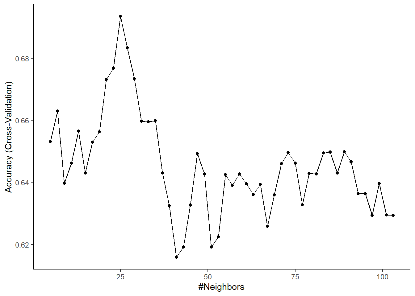
You can also set the candidate values of the hyperparameter directly rather than having Caret select them
NOTE: tune_grid dataframe & assignment of it to \(tuneGrid\) argument
tc_kfold <- trainControl(method = "cv", number = 10,
                         savePredictions = TRUE, classProbs = TRUE)

tune_grid <- expand.grid(k = seq(1,150, by = 2))

set.seed(20140102)
m_kfold_knn_grid <- train(x = all_x, y = all_y,
                       method = "knn",
                       trControl = tc_kfold,
                       tuneGrid = tune_grid)

m_kfold_knn_grid
## k-Nearest Neighbors
##
## 297 samples
## 16 predictor
## 2 classes: 'no', 'yes'
##
## No pre-processing
## Resampling: Cross-Validated (10 fold)
## Summary of sample sizes: 268, 267, 268, 267, 267, 267, ...
## Resampling results across tuning parameters:
##
## k Accuracy Kappa
## 1 0.5658621 0.1261572
## 3 0.6331034 0.2591963
## 5 0.6497701 0.2883933
## 7 0.6629885 0.3174775
## 9 0.6397701 0.2704719
## 11 0.6462069 0.2847430
## 13 0.6565517 0.3042528
## 15 0.6429885 0.2782284
## 17 0.6529885 0.2967799
## 19 0.6563218 0.3033552
## 21 0.6731034 0.3396912
## 23 0.6767816 0.3456311
## 25 0.6934483 0.3776990
## 27 0.6833333 0.3587564
## 29 0.6734483 0.3372818
## 31 0.6596552 0.3059844
## 33 0.6595402 0.3063698
## 35 0.6598851 0.3073338
## 37 0.6429885 0.2735483
## 39 0.6325287 0.2493264
## 41 0.6158621 0.2134469
## 43 0.6191954 0.2192097
## 45 0.6326437 0.2469868
## 47 0.6493103 0.2810765
## 49 0.6427586 0.2680136
## 51 0.6191954 0.2196535
## 53 0.6224138 0.2246722
## 55 0.6425287 0.2652431
## 57 0.6390805 0.2569110
## 59 0.6427586 0.2643655
## 61 0.6395402 0.2596664
## 63 0.6360920 0.2516933
## 65 0.6393103 0.2557566
## 67 0.6293103 0.2340220
## 69 0.6359770 0.2480220
## 71 0.6459770 0.2686925
## 73 0.6495402 0.2755113
## 75 0.6462069 0.2681505
## 77 0.6327586 0.2406470
## 79 0.6428736 0.2604854
## 81 0.6427586 0.2599318
## 83 0.6494253 0.2737088
## 85 0.6497701 0.2742781
## 87 0.6429885 0.2608585
## 89 0.6498851 0.2750210
## 91 0.6465517 0.2678604
## 93 0.6363218 0.2471627
## 95 0.6363218 0.2465400
## 97 0.6294253 0.2327520
## 99 0.6396552 0.2536947
## 101 0.6295402 0.2324664
## 103 0.6294253 0.2315603
## 105 0.6159770 0.2044791
## 107 0.6227586 0.2175998
## 109 0.6294253 0.2296145
## 111 0.6191954 0.2096740
## 113 0.6293103 0.2293822
## 115 0.6327586 0.2360654
## 117 0.6259770 0.2221558
## 119 0.6294253 0.2274579
## 121 0.6295402 0.2276303
## 123 0.6363218 0.2409151
## 125 0.6398851 0.2492272
## 127 0.6398851 0.2485254
## 129 0.6432184 0.2550605
## 131 0.6500000 0.2683212
## 133 0.6397701 0.2463055
## 135 0.6397701 0.2433937
## 137 0.6432184 0.2514192
## 139 0.6432184 0.2507187
## 141 0.6365517 0.2360585
## 143 0.6365517 0.2351484
## 145 0.6329885 0.2290710
## 147 0.6431034 0.2475315
## 149 0.6366667 0.2338132
##
## Accuracy was used to select the optimal model using the largest value.
## The final value used for the model was k = 25.You can plot performance by K again for this set of model configurations
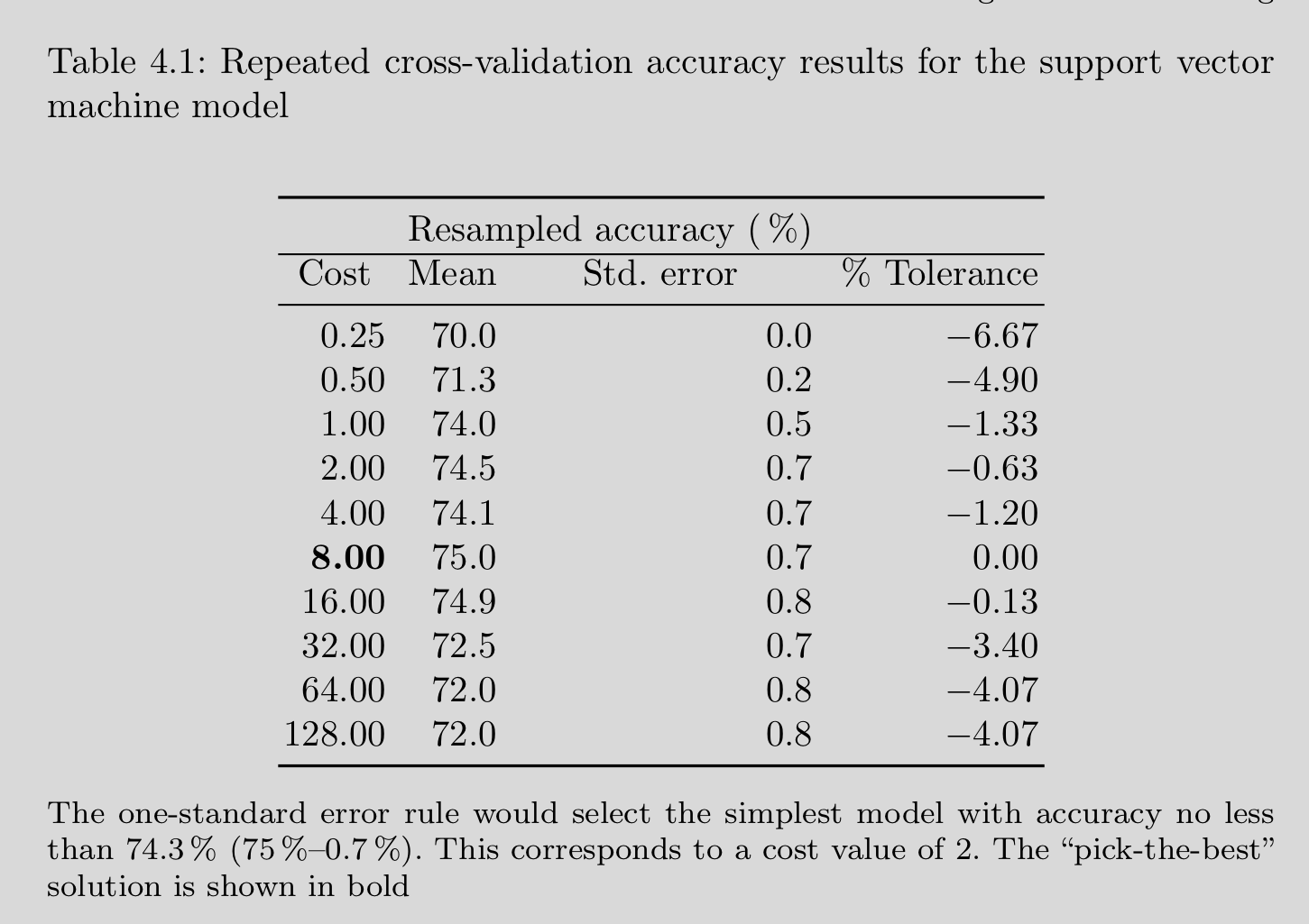
The simplest way to select among model configurations (e.g., hyperparameters) is to choose the model configuration with the best performance
There are other methods. Next most common is to choose the simplest (least flexible) model that has performance within one SE of the best performing configuration. Kuhn also describes an option of selecting using a tolerance relative to the best performing model.
Caret help provides more detail about how to use these two alternative selection methods for hyperparameter tuning
4.9 Caret Pre-processing within CV
Lets look again at our 10-fold CV for tuning the knn model from earlier.
What did we forget to do that is necessary when using knn models?
- We didn’t scale our predictors.
tc_kfold <- trainControl(method = "cv", number = 10,
                         savePredictions = TRUE, classProbs = TRUE)

set.seed(20140102)
m_kfold_knn <- train(x = all_x, y = all_y,
                     method = "knn",
                     trControl = tc_kfold,
                     tuneLength = 50)
How did we handle data preprocessing that uses info from the dataset (e.g., missing value imputation, range correction, other transformations) in the single validation set CV approach?
- We only used training data to make decisions about the values for the preprocessing. We then applied these same values from training for the pre-processing of test data
How would this generalize to other CV methods such as K-fold CV?
- We will need to get multiple estimates of these pre-processing values from each set of held-in/training set and apply separately to each associated held-out test set. We could do this manually if we handled the iterations in a for loop. However, if we are going to let Caret do the CV looping for us, we need to use its internal preprocessing functions
You should read on pre-processing in Caret to get a sense of the full scope of what is available.
There are a handful of stand alone pre-processing functions but most methods should be implemented within \(preProcess()\). See its help
- Distributional transformations including “BoxCox”, “YeoJohnson”, “expoTrans”, “spatialSign”
- Scaling including “center”, “scale”, “range”
- Data imputation including “knnImpute”, “bagImpute”, “medianImpute”
- Identification of low variance predictors including “zv”, “nzv”, and “conditionalX”
- Identification (and removal) of highly correlated predictors using “corr”
- Dimensionality reductions including “pca”, “ica”
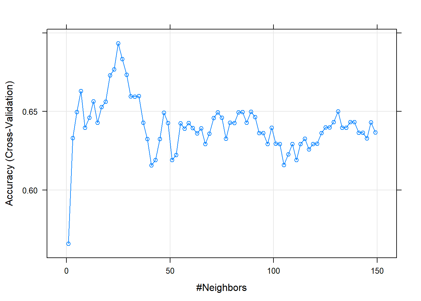
Lets do K-fold with knn properly
Lets return to the original dataset with the nzv variable and some missing data too
dmy <- dummyVars(~ ., data = d_all, sep = "_", fullRank = TRUE)

d <- as_tibble(predict(dmy, d_all)) %>%
  select(-disease_yes) %>%
  mutate(disease = d_all$disease) %>%
  glimpse()
## Observations: 303
## Variables: 18
## $ age <dbl> 63, 67, 67, 37, 41, 56, 62, 57, 63, 53, 5…
## $ sex_male <dbl> 1, 1, 1, 1, 0, 1, 0, 0, 1, 1, 1, 0, 1, 1,…
## $ cp_atypicalangina <dbl> 0, 0, 0, 0, 1, 1, 0, 0, 0, 0, 0, 1, 0, 1,…
## $ cp_nonanginalpain <dbl> 0, 1, 1, 1, 0, 0, 1, 1, 1, 1, 1, 0, 1, 0,…
## $ rest_bp <dbl> 145, 160, 120, 130, 130, 120, 140, 120, 1…
## $ chol <dbl> 233, 286, 229, 250, 204, 236, 268, 354, 2…
## $ fbs_True <dbl> 1, 0, 0, 0, 0, 0, 0, 0, 0, 1, 0, 0, 1, 0,…
## $ rest_ecg_sttwaveabnormality <dbl> 0, 0, 0, 0, 0, 0, 0, 0, 0, 0, 0, 0, 0, 0,…
## $ rest_ecg_leftventricularhypertrophymax <dbl> 1, 1, 1, 0, 1, 0, 1, 0, 1, 1, 0, 1, 1, 0,…
## $ max_hr <dbl> 150, 108, 129, 187, 172, 178, 160, 163, 1…
## $ ex_ang_yes <dbl> 0, 1, 1, 0, 0, 0, 0, 1, 0, 1, 0, 0, 1, 0,…
## $ ex_st_depress <dbl> 2.3, 1.5, 2.6, 3.5, 1.4, 0.8, 3.6, 0.6, 1…
## $ ex_st_slope_flat <dbl> 0, 1, 1, 0, 0, 0, 0, 0, 1, 0, 1, 1, 1, 0,…
## $ ex_st_slope_downslope <dbl> 1, 0, 0, 1, 0, 0, 1, 0, 0, 1, 0, 0, 0, 0,…
## $ ca <dbl> 0, 3, 2, 0, 0, 0, 2, 0, 1, 0, 0, 0, 1, 0,…
## $ thal_fixeddefect <dbl> 1, 0, 0, 0, 0, 0, 0, 0, 0, 0, 1, 0, 1, 0,…
## $ thal_reversabledefect <dbl> 0, 0, 1, 0, 0, 0, 0, 0, 1, 1, 0, 0, 0, 1,…
## $ disease <fct> no, yes, yes, no, no, no, yes, no, yes, y…Note that preProcess() is handled within \(train()\) not \(trainControl()\) because you might do different pre-processing steps for different statistical algorithms
We will
- remove nzv variables
- median impute
- range correct
tc_kfold <- trainControl(method = "cv", number = 10,
savePredictions = TRUE, classProbs = TRUE)
set.seed(20140102)
m_kfold_pre <- train(x = all_x, y = all_y,
method = "knn",
trControl = tc_kfold,
tuneLength = 50,
preProcess = c("range", "nzv", "medianImpute"))Lets see what Caret did
## k-Nearest Neighbors
##
## 303 samples
## 17 predictor
## 2 classes: 'no', 'yes'
##
## Pre-processing: re-scaling to [0, 1] (16), median imputation (16), remove (1)
## Resampling: Cross-Validated (10 fold)
## Summary of sample sizes: 273, 273, 272, 273, 272, 273, ...
## Resampling results across tuning parameters:
##
## k Accuracy Kappa
## 5 0.8082796 0.6124460
## 7 0.8248387 0.6445448
## 9 0.8213978 0.6382924
## 11 0.8116129 0.6166102
## 13 0.8049462 0.6021256
## 15 0.8116129 0.6163001
## 17 0.8017204 0.5955917
## 19 0.8017204 0.5955917
## 21 0.8016129 0.5968425
## 23 0.8082796 0.6097569
## 25 0.8049462 0.6027208
## 27 0.8049462 0.6023045
## 29 0.8016129 0.5959329
## 31 0.8113978 0.6153170
## 33 0.8115054 0.6153240
## 35 0.8081720 0.6081468
## 37 0.8048387 0.6014206
## 39 0.8081720 0.6079854
## 41 0.7982796 0.5875124
## 43 0.8016129 0.5940618
## 45 0.8082796 0.6082798
## 47 0.8049462 0.6017048
## 49 0.8050538 0.6020054
## 51 0.8116129 0.6152672
## 53 0.8083871 0.6085481
## 55 0.8083871 0.6084927
## 57 0.8116129 0.6152119
## 59 0.8083871 0.6084927
## 61 0.8083871 0.6084927
## 63 0.8117204 0.6151591
## 65 0.8117204 0.6151591
## 67 0.8150538 0.6217341
## 69 0.8150538 0.6217341
## 71 0.8117204 0.6151319
## 73 0.8117204 0.6151319
## 75 0.8083871 0.6084655
## 77 0.8149462 0.6217869
## 79 0.8149462 0.6218510
## 81 0.8149462 0.6218510
## 83 0.8149462 0.6218510
## 85 0.8116129 0.6154794
## 87 0.8116129 0.6154794
## 89 0.8116129 0.6154794
## 91 0.8116129 0.6154794
## 93 0.8082796 0.6091638
## 95 0.8082796 0.6091638
## 97 0.8117204 0.6170549
## 99 0.8149462 0.6235059
## 101 0.8181720 0.6289606
## 103 0.8215054 0.6355628
##
## Accuracy was used to select the optimal model using the largest value.
## The final value used for the model was k = 7.From help for \(preProcess()\)
The operations are applied in this order: zero-variance filter, near-zero variance filter, correlation filter, Box-Cox/Yeo-Johnson/exponential transformation, centering, scaling, range, imputation, PCA, ICA then spatial sign.
If PCA is requested but centering and scaling are not, the values will still be centered and scaled. Similarly, when ICA is requested, the data are automatically centered and scaled.
k-nearest neighbor imputation is carried out by finding the k closest samples (Euclidian distance) in the training set. Imputation via bagging fits a bagged tree model for each predictor (as a function of all the others). This method is simple, accurate and accepts missing values, but it has much higher computational cost. Imputation via medians takes the median of each predictor in the training set, and uses them to fill missing values. This method is simple, fast, and accepts missing values, but treats each predictor independently, and may be inaccurate.
A warning is thrown if both PCA and ICA are requested. ICA, as implemented by the fastICA package automatically does a PCA decomposition prior to finding the ICA scores.
The function will throw an error of any numeric variables in x has less than two unique values unless either method = “zv” or method = “nzv” are invoked.
Non-numeric data will not be pre-processed and there values will be in the data frame produced by the predict function. Note that when PCA or ICA is used, the non-numeric columns may be in different positions when predicted.
Now knn is working much better!
## [1] 0.6934483## [1] 0.82483874.10 Training, Validation, and Test
Cross validation can be used to select the best model configuration and/or evaluate model performance.
What is the problem with doing both simultaneously?
- If you use your held-out samples to select the best model then the same held out samples can not also be used to evaluate the performance of that same best model. If it is, the performance metric will have ‘optimization bias’. To the degree that there is any noise (i.e., variance) in the measurement of performance, selecting the best model configuration will capitalize on this noise.
What is the solution to this problem?
- You need to use one set of held out sample(s) to select the best model. Then you need a DIFFERENT set of held out sample(s) to evaluate that best model. There are two strategies for this: 1) training, validation, test method or 2) nested cross validation.
NOTES:
- Simple (single loop) CV methods with the full sample are still common
- Failure by some (even Kuhn) to appreciate the degree of optimization bias
- Particular problem in Psychology because of small n (high variance in our performance metric)?
Training, Validation and Test
First divide your data into training and test
Do some form of CV using the training data to select the best model configuration. E.g., -
- Further divide training into separate training and validation sets
- K-fold using training
- Bootstrap CV using training
After you select the best model configuration using CV in the training set
Refit that model configuration in the FULL training set
Evaluate it in the test set
Of course, in the end, you will refit this final model configuration to the FULL dataset but the performance estimate will come from test only
- Use \(initial\_split()\) for first train/test split
- Use trn data for CV (in this case bootstrap; Why bootstrap?)
set.seed(20140102)
splits <- initial_split(d, prop = .75, strata = "disease")
trn <- training(splits)
test <- testing(splits)
trn_x <- trn %>%
select(-disease) %>%
as.data.frame()
trn_y <- trn %>%
pull(disease)
tc_boot <- trainControl(method = "boot", number = 100,
savePredictions = TRUE, classProbs = TRUE)
m_boot_cv <- train(x = trn_x, y = trn_y,
method = "knn",
trControl = tc_boot,
tuneLength = 50,
preProcess = c("range", "nzv", "medianImpute"))This is the best model determined by bootstrap CV
BUT this is NOT the correct estimate of its performance
We compared 50 model configurations (values of k). This performance estimate will have some optimalization bias
## k-Nearest Neighbors
##
## 228 samples
## 17 predictor
## 2 classes: 'no', 'yes'
##
## Pre-processing: re-scaling to [0, 1] (16), median imputation (16), remove (1)
## Resampling: Bootstrapped (100 reps)
## Summary of sample sizes: 228, 228, 228, 228, 228, 228, ...
## Resampling results across tuning parameters:
##
## k Accuracy Kappa
## 5 0.7831911 0.5613646
## 7 0.7931133 0.5807077
## 9 0.7949809 0.5839535
## 11 0.7957481 0.5853539
## 13 0.7938318 0.5812652
## 15 0.7946406 0.5824852
## 17 0.7938674 0.5807068
## 19 0.7944408 0.5821319
## 21 0.7921254 0.5773930
## 23 0.7927796 0.5786146
## 25 0.7920921 0.5774580
## 27 0.7921601 0.5774438
## 29 0.7947046 0.5826322
## 31 0.7933862 0.5798220
## 33 0.7928604 0.5785610
## 35 0.7918744 0.5766039
## 37 0.7921804 0.5771260
## 39 0.7907577 0.5741414
## 41 0.7916017 0.5757700
## 43 0.7909449 0.5741373
## 45 0.7907964 0.5739057
## 47 0.7899280 0.5719896
## 49 0.7914243 0.5750783
## 51 0.7918117 0.5757517
## 53 0.7951774 0.5825886
## 55 0.7944286 0.5812386
## 57 0.7931171 0.5785282
## 59 0.7945334 0.5814117
## 61 0.7939141 0.5801716
## 63 0.7948753 0.5819970
## 65 0.7957588 0.5838967
## 67 0.7949985 0.5823159
## 69 0.7967126 0.5858995
## 71 0.7947992 0.5820313
## 73 0.7961449 0.5848659
## 75 0.7939766 0.5806345
## 77 0.7932741 0.5793905
## 79 0.7927730 0.5783271
## 81 0.7901244 0.5732910
## 83 0.7891700 0.5713997
## 85 0.7903778 0.5742762
## 87 0.7872661 0.5677890
## 89 0.7885137 0.5701963
## 91 0.7888588 0.5708184
## 93 0.7884870 0.5700831
## 95 0.7881026 0.5693142
## 97 0.7868214 0.5666661
## 99 0.7861636 0.5654327
## 101 0.7871431 0.5672339
## 103 0.7856813 0.5642872
##
## Accuracy was used to select the optimal model using the largest value.
## The final value used for the model was k = 69.## [1] 0.7967126We need to train a k = 13 model in all of training and then use that model to predict in test
- Caret already re-trained the model using all of the data in trn for us
We just need to use it to make predictions in test and then evaluate those predictions
- Our model object already knows all the pre-processing we did and what the appropriate trn values are too.
We love Caret!
## Confusion Matrix and Statistics
##
## Reference
## Prediction no yes
## no 36 6
## yes 5 28
##
## Accuracy : 0.8533
## 95% CI : (0.7527, 0.9244)
## No Information Rate : 0.5467
## P-Value [Acc > NIR] : 1.664e-08
##
## Kappa : 0.7033
##
## Mcnemar's Test P-Value : 1
##
## Sensitivity : 0.8235
## Specificity : 0.8780
## Pos Pred Value : 0.8485
## Neg Pred Value : 0.8571
## Prevalence : 0.4533
## Detection Rate : 0.3733
## Detection Prevalence : 0.4400
## Balanced Accuracy : 0.8508
##
## 'Positive' Class : yes
## 4.11 Nested Cross Validation
The training, validation, and test method to simultaneously select and evaluate models is commonly used
However, it suffers from the same problems as the single validation set approach
- Only a single small held out test set (high variance/imprecise estimate of model performance)
- Biased estimate of model performance (training uses only 50 - 80% of data)
Nested CV is emerging as a preferred solution
Nested CV invovles nested \(for\) loops (but we can let Caret handle the inner loop like we did for single loop CV)
Nested CV is VERY CONFUSING at first (like the first year you use it!)
A ‘simple’ example using bootstrap for inner loop and 10-fold for outer loop
- Divide the full sample into 10 folds
- Iterate through those 10 folds as follows (this is the outer loop)
- Hold out fold 1
- Use folds 2-10 to do the inner loop CV
- Bootstrap these folds B times
- Fit models to B bootstrap samples
- Calculate selection performance metrics in B out-of-bag samples
- Average the B bootstrapped selection performance metrics for each model configuration
- Select the best model configuration using this average bootstrapped selection performance metric
- Use best model configuration from folds 2-10 to make predictions for the held-out fold 1 to get the first (of ten) evaluation performance metrics
- Repeat for held out fold 2 - 10
- Average the 10 evaluation performance metrics. This is the expected performance of a best model configuration (selected by B bootstraps) in new data. [You still dont know what configruation you should use because you have 10 ‘best’ model configurations]
- Do B bootstraps with the full sample to select the best model configuration
- Fit this best model configuration to the full data
TRY TO DRAW THIS ON BOARD
Here is an example of one way to code this to run on a single (multi-core?) machine
set.seed(20140102)
outer <- vfold_cv(d, v = 10, repeats = 1, strata = "disease")
tc_boot <- trainControl(method = "boot", number = 100,
savePredictions = TRUE, classProbs = TRUE)
results <- tibble(fold = numeric(),
k = numeric(),
acc_test = numeric())
for (i in seq_along(outer$splits)) {
trn_x <- outer$splits[[i]] %>%
analysis() %>%
select(-disease) %>%
as.data.frame()
trn_y <- outer$splits[[i]] %>%
analysis() %>%
pull(disease)
test <- outer$splits[[i]] %>%
assessment()
#Caret handles inner loop to select by bootstrap
m_inner <- train(x = trn_x, y = trn_y,
method = "knn",
trControl = tc_boot,
tuneLength = 50,
preProcess = c("range", "nzv", "medianImpute"))
#predictions in held-out fold from outer loop
acc <- confusionMatrix(predict(m_inner, test), test$disease, positive = "yes")
results <- add_row(results,
fold = i,
k = as.numeric(m_inner$bestTune),
acc_test = acc$overall["Accuracy"])
}Models that are trained in 90% of the data and selected by 50 bootstraps have this performance in 10% held-out folds
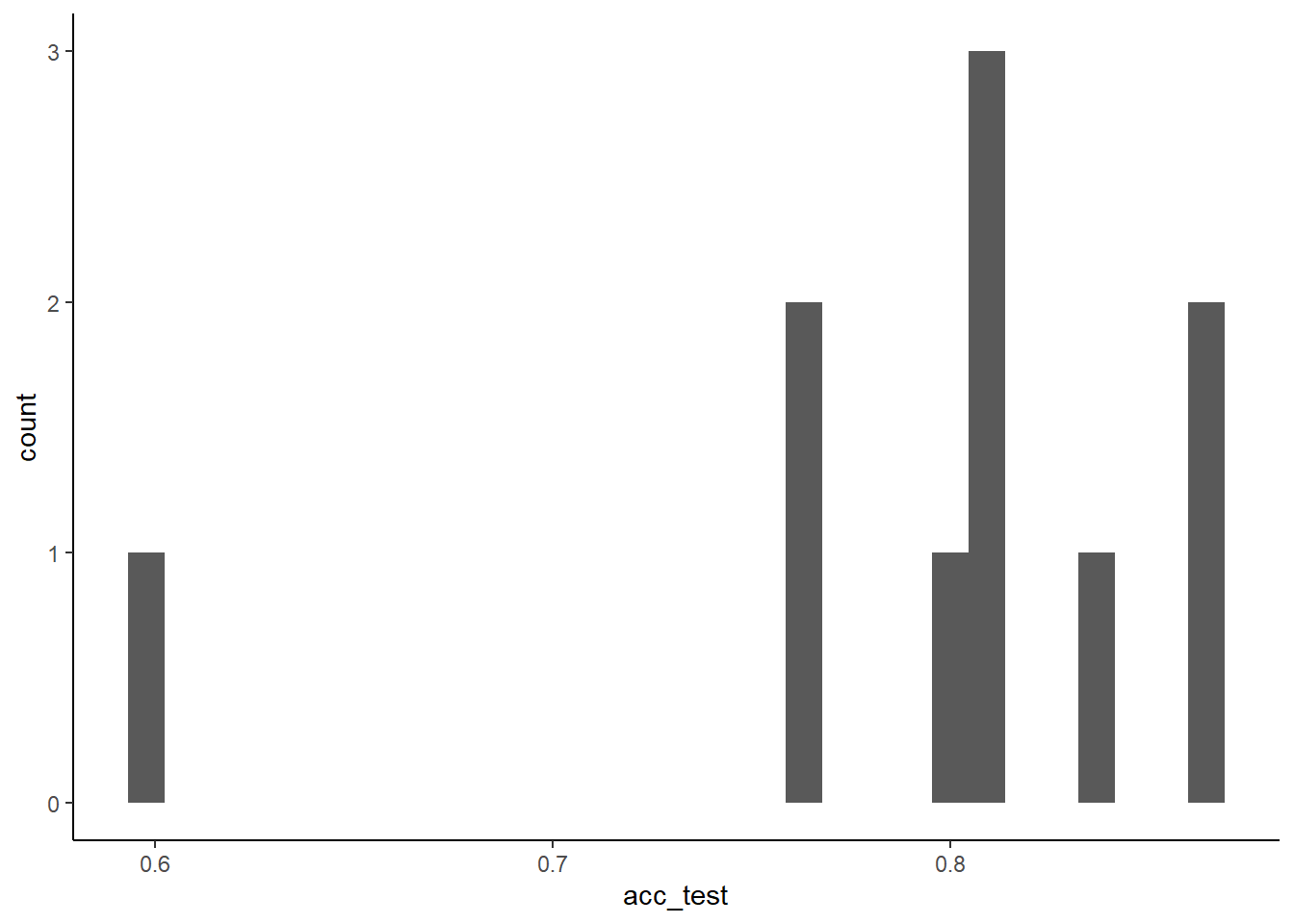
## [1] 0.7920133## [1] 0.0756488Nested CV evaluates a training/selection process not a model configuration!
You therefore need to select a final model configuration using same CV with full data
You then need to fit that new model configuration to the full data
Single loop bootstrap CV with the full data using Caret will do both of these steps
all_x <- d %>%
  select(-disease) %>%
  as.data.frame()

all_y <- d %>%
  pull(disease)
tc_boot <- trainControl(method = "boot", number = 100,
savePredictions = TRUE, classProbs = TRUE)
m_inner <- train(x = all_x, y = all_y,
method = "knn",
trControl = tc_boot,
tuneLength = 50,
preProcess = c("range", "nzv", "medianImpute"))
m_inner$bestTune## k
## 48 99Why bootstrap on inner loop and k-fold on outer loop?
- The inner loop is used for selecting models. Bootstrap yields low variance performance estimates (but they are biased). We want low variance to select best model configuration. K-fold is a good method for less biased performance estimates. We want less bias in our final evaluation of our best model. You can do repeated K-fold to both reduce its variance and give you a sense of the performance sampling distribution.
4.12 Alternative Performance Metrics in \(train()\)
You can select models during cross validation with performance metrics other than accuracy
You should generally use the performance metric that is the best aligned with your problem and/or most clear to your audience
- In classification
- Do you care about types of errors or just overall error rate
- Is the outcome relatively balanced or unbalanced
- In regression
- Which metric is most accessible to your audience
- Do you want to weight big and small errors the same
Here is an example of single loop CV (100 bootstraps) for model selection using Area under the ROC curve
You can also develop your own alternative performance metric
NOTE: Use of different \(summaryFunction\)
tc_boot_auc <- trainControl(method = "boot", number = 100,
                        summaryFunction = twoClassSummary,
                        savePredictions = TRUE, classProbs = TRUE)

set.seed(20140102)
m_auc <- train(x = all_x, y = all_y,
               method = "knn",
               trControl = tc_boot_auc,
               tuneLength = 50,
               metric = "ROC",
               preProcess = c("range", "nzv", "medianImpute"))

m_auc
## k-Nearest Neighbors
##
## 303 samples
## 17 predictor
## 2 classes: 'no', 'yes'
##
## Pre-processing: re-scaling to [0, 1] (16), median imputation (16), remove (1)
## Resampling: Bootstrapped (100 reps)
## Summary of sample sizes: 303, 303, 303, 303, 303, 303, ...
## Resampling results across tuning parameters:
##
## k ROC Sens Spec
## 5 0.8449642 0.8131412 0.7480645
## 7 0.8593345 0.8218229 0.7593982
## 9 0.8681028 0.8337427 0.7567340
## 11 0.8749687 0.8427924 0.7564068
## 13 0.8769052 0.8462298 0.7541010
## 15 0.8774478 0.8480513 0.7537166
## 17 0.8774627 0.8536673 0.7494302
## 19 0.8775834 0.8511416 0.7481818
## 21 0.8757533 0.8517993 0.7475717
## 23 0.8745625 0.8521122 0.7430370
## 25 0.8747110 0.8551845 0.7408166
## 27 0.8742510 0.8550312 0.7427486
## 29 0.8743935 0.8561414 0.7410196
## 31 0.8740498 0.8528986 0.7425977
## 33 0.8736163 0.8580450 0.7426338
## 35 0.8751786 0.8609552 0.7430037
## 37 0.8753934 0.8590479 0.7435483
## 39 0.8768434 0.8599029 0.7418648
## 41 0.8775216 0.8615812 0.7401394
## 43 0.8779709 0.8642704 0.7395705
## 45 0.8791269 0.8675705 0.7385684
## 47 0.8796417 0.8687995 0.7365295
## 49 0.8805505 0.8679567 0.7346352
## 51 0.8804160 0.8679718 0.7320861
## 53 0.8813101 0.8681030 0.7313360
## 55 0.8821149 0.8704670 0.7285919
## 57 0.8825020 0.8715123 0.7301339
## 59 0.8826171 0.8710996 0.7293672
## 61 0.8827661 0.8744207 0.7298689
## 63 0.8828698 0.8719576 0.7292197
## 65 0.8829120 0.8720771 0.7299217
## 67 0.8828011 0.8719851 0.7286233
## 69 0.8833760 0.8709146 0.7283048
## 71 0.8835409 0.8727288 0.7294953
## 73 0.8835545 0.8739133 0.7289782
## 75 0.8831506 0.8732926 0.7263126
## 77 0.8831483 0.8741307 0.7273924
## 79 0.8831137 0.8735851 0.7279831
## 81 0.8834780 0.8736621 0.7267663
## 83 0.8833970 0.8749416 0.7275635
## 85 0.8832693 0.8741780 0.7305023
## 87 0.8828591 0.8749010 0.7300265
## 89 0.8830617 0.8755645 0.7298228
## 91 0.8833481 0.8768744 0.7311682
## 93 0.8835018 0.8795365 0.7300335
## 95 0.8833482 0.8788290 0.7301809
## 97 0.8833099 0.8776563 0.7302421
## 99 0.8834794 0.8777261 0.7306612
## 101 0.8838177 0.8767995 0.7323063
## 103 0.8839166 0.8771182 0.7315643
##
## ROC was used to select the optimal model using the largest value.
## The final value used for the model was k = 103.4.13 Data Exploration in a Nested World….
Final words on cross validation:
Iterative methods (K-fold, boostrap) are superior to single validation set approach wrt bias-variance trade-off in performance measurement
Nested or train, validation, test set approach should be used when you plan to both select among model configurations AND evaluate the best model
Iterative methods (and Nested itereative methods in particular) must be handled very carefully wrt data exploration b/c they use all the data
- Can use eyeball sample (10% of data) without much affect on performance measurement
- If you plan to do a lot of exploration (e.g., lots of feature engineering and feature selection), maybe use single validation (or train, test, validation)