2 Introduction to Regression Models
Introduction to key instructional dataset: Ames Housing Prices
Use of root mean square error (RMSE) in training and test sets for model performance evaluation
The General Linear Model as a machine learning model
- Extensions to categorical variables
- Dummy coding
- One-hot coding
- Extensions to interactive and non-linear effects of predictors
- Extensions to categorical variables
K Nearest Neighbour (KNN)
- Hyperparameter k
- Normalization of predictors
- Extensions to categorical variables
2.1 The Ames Housing Prices Dataset
We will use the Ames Housing Prices dataset as a running example this unit (and some future units and homeworks as well)
You can read more about the original dataset created by Dean DeCock
This dataset is now hosted by Kaggle
- Kaggle is an online community of data scientists and machine learners.
- It allows users to find and publish data sets, explore and build models, compete for best models, and share documented solutions
- We will use Kaggle a lot. Its a great resource.
The data set contains data from home sales in sale of individual residential property in Ames, Iowa from 2006 to 2010
The original data set includes 2930 observations of sales price and a large number of explanatory variables (23 nominal, 23 ordinal, 14 discrete, and 20 continuous)
Here is the original codebook from Kaggle
For the competition, Kaggle provides us with a dataset that includes 1460 observations. Kaggle retained the remaining observations to evaluate model performance for models submitted to its competition.
Why?
- Models may become very overfit to the datasest they give us through comparing many, many different model configurations by brute force. The true metric for how well a model performs is its performance in new data that it hasnt seen. They make sure that developers have never seen these new data by not making it available to the developers.
Our goal is to build a machine learning model that predicts the sale price for houses from future sales
To begin this project we need to:
- Load the packages we will need
- Open the data
- Tidy the variable names
NOTE: redefine \(select()\) because of \(MASS\) package conflict
library(caret)
library(tidyverse)
library(janitor)

select <- dplyr::select

data_path <- "data"
ames <- read_csv(file.path(data_path, "ames.csv")) %>%
  clean_names(case = "snake") %>%
  select(-id)
We will also make a tibble to track training and test error across the models we fit
## Observations: 0
## Variables: 3
## $ model      <chr>
## $ rmse_train <dbl>
## $ rmse_test  <dbl>
We will fit various regression models to the data. These will include:
- Simple linear regression
- Multiple regression
- Multiple regressions with interactions, transformations, polynomial predictors
- K Nearest Neighbour (KNN), a non-parametric model
To fit and then evaluate/compare these models, we need training and test data
Why?
- Once again, these models will differ in how much they overfit the training set. As p increases, as we include polynomials and interactions, and as we move to non-parametric models, these models will fit training well but perhaps only by fitting the noise. As such, they may not work well with new data. We need new data to evaluate that.
To build models that will work well in new data (e.g., the data that Kaggle has retained from us):
We can split the dataset Kaggle gave to us (N=1460) into a private training and test set for our own use
We will fit models in train
We will evaluate them in test
Can use an 80/20 split using rsample package
Can stratify on the outcome
Here is the code
- Note the use of \(set.seed()\) to get reproducible splits
library(rsample)

set.seed(19690127)
ames_splits <- initial_split(ames, prop = .8, strata = "sale_price")

train_all <- training(ames_splits)
test <- testing(ames_splits)
This results in N = 1170 in train and N = 290 in test
## [1] 1170 80## [1] 290 80Lets take a quick look at the available variables in the training data
## Observations: 1,170
## Variables: 80
## $ ms_sub_class    <dbl> 60, 60, 50, 20, 50, 190, 20, 20, 20, 45, 90, 20, 20, 60, 45, 20,…
## $ ms_zoning       <chr> "RL", "RL", "RL", "RL", "RM", "RL", "RL", "RL", "RL", "RM", "RL"…
## $ lot_frontage    <dbl> 65, 68, 85, 75, 51, 50, 70, NA, NA, 51, 72, 66, 70, 101, 57, 75,…
## $ lot_area        <dbl> 8450, 11250, 14115, 10084, 6120, 7420, 11200, 12968, 10920, 6120…
## $ street          <chr> "Pave", "Pave", "Pave", "Pave", "Pave", "Pave", "Pave", "Pave", …
## $ alley           <chr> NA, NA, NA, NA, NA, NA, NA, NA, NA, NA, NA, NA, NA, NA, "Grvl", …
## $ lot_shape       <chr> "Reg", "IR1", "IR1", "Reg", "Reg", "Reg", "Reg", "IR2", "IR1", "…
## $ land_contour    <chr> "Lvl", "Lvl", "Lvl", "Lvl", "Lvl", "Lvl", "Lvl", "Lvl", "Lvl", "…
## $ utilities       <chr> "AllPub", "AllPub", "AllPub", "AllPub", "AllPub", "AllPub", "All…
## $ lot_config      <chr> "Inside", "Inside", "Inside", "Inside", "Inside", "Corner", "Ins…
## $ land_slope      <chr> "Gtl", "Gtl", "Gtl", "Gtl", "Gtl", "Gtl", "Gtl", "Gtl", "Gtl", "…
## $ neighborhood    <chr> "CollgCr", "CollgCr", "Mitchel", "Somerst", "OldTown", "BrkSide"…
## $ condition1      <chr> "Norm", "Norm", "Norm", "Norm", "Artery", "Artery", "Norm", "Nor…
## $ condition2      <chr> "Norm", "Norm", "Norm", "Norm", "Norm", "Artery", "Norm", "Norm"…
## $ bldg_type       <chr> "1Fam", "1Fam", "1Fam", "1Fam", "1Fam", "2fmCon", "1Fam", "1Fam"…
## $ house_style     <chr> "2Story", "2Story", "1.5Fin", "1Story", "1.5Fin", "1.5Unf", "1St…
## $ overall_qual    <dbl> 7, 7, 5, 8, 7, 5, 5, 5, 6, 7, 4, 5, 5, 8, 7, 8, 5, 5, 8, 5, 8, 5…
## $ overall_cond    <dbl> 5, 5, 5, 5, 5, 6, 5, 6, 5, 8, 5, 5, 6, 5, 7, 5, 7, 8, 5, 7, 5, 6…
## $ year_built      <dbl> 2003, 2001, 1993, 2004, 1931, 1939, 1965, 1962, 1960, 1929, 1967…
## $ year_remod_add  <dbl> 2003, 2002, 1995, 2005, 1950, 1950, 1965, 1962, 1960, 2001, 1967…
## $ roof_style      <chr> "Gable", "Gable", "Gable", "Gable", "Gable", "Gable", "Hip", "Hi…
## $ roof_matl       <chr> "CompShg", "CompShg", "CompShg", "CompShg", "CompShg", "CompShg"…
## $ exterior1st     <chr> "VinylSd", "VinylSd", "VinylSd", "VinylSd", "BrkFace", "MetalSd"…
## $ exterior2nd     <chr> "VinylSd", "VinylSd", "VinylSd", "VinylSd", "Wd Shng", "MetalSd"…
## $ mas_vnr_type    <chr> "BrkFace", "BrkFace", "None", "Stone", "None", "None", "None", "…
## $ mas_vnr_area    <dbl> 196, 162, 0, 186, 0, 0, 0, 0, 212, 0, 0, 0, 0, 380, 0, 281, 0, 0…
## $ exter_qual      <chr> "Gd", "Gd", "TA", "Gd", "TA", "TA", "TA", "TA", "TA", "TA", "TA"…
## $ exter_cond      <chr> "TA", "TA", "TA", "TA", "TA", "TA", "TA", "TA", "TA", "TA", "TA"…
## $ foundation      <chr> "PConc", "PConc", "Wood", "PConc", "BrkTil", "BrkTil", "CBlock",…
## $ bsmt_qual       <chr> "Gd", "Gd", "Gd", "Ex", "TA", "TA", "TA", "TA", "TA", "TA", NA, …
## $ bsmt_cond       <chr> "TA", "TA", "TA", "TA", "TA", "TA", "TA", "TA", "TA", "TA", NA, …
## $ bsmt_exposure   <chr> "No", "Mn", "No", "Av", "No", "No", "No", "No", "No", "No", NA, …
## $ bsmt_fin_type1  <chr> "GLQ", "GLQ", "GLQ", "GLQ", "Unf", "GLQ", "Rec", "ALQ", "BLQ", "…
## $ bsmt_fin_sf1    <dbl> 706, 486, 732, 1369, 0, 851, 906, 737, 733, 0, 0, 646, 504, 0, 0…
## $ bsmt_fin_type2  <chr> "Unf", "Unf", "Unf", "Unf", "Unf", "Unf", "Unf", "Unf", "Unf", "…
## $ bsmt_fin_sf2    <dbl> 0, 0, 0, 0, 0, 0, 0, 0, 0, 0, 0, 0, 0, 0, 0, 0, 0, 668, 0, 486, …
## $ bsmt_unf_sf     <dbl> 150, 434, 64, 317, 952, 140, 134, 175, 520, 832, 0, 468, 525, 11…
## $ total_bsmt_sf   <dbl> 856, 920, 796, 1686, 952, 991, 1040, 912, 1253, 832, 0, 1114, 10…
## $ heating         <chr> "GasA", "GasA", "GasA", "GasA", "GasA", "GasA", "GasA", "GasA", …
## $ heating_qc      <chr> "Ex", "Ex", "Ex", "Ex", "Gd", "Ex", "Ex", "TA", "TA", "Ex", "TA"…
## $ central_air     <chr> "Y", "Y", "Y", "Y", "Y", "Y", "Y", "Y", "Y", "Y", "Y", "Y", "Y",…
## $ electrical      <chr> "SBrkr", "SBrkr", "SBrkr", "SBrkr", "FuseF", "SBrkr", "SBrkr", "…
## $ x1st_flr_sf     <dbl> 856, 920, 796, 1694, 1022, 1077, 1040, 912, 1253, 854, 1296, 111…
## $ x2nd_flr_sf     <dbl> 854, 866, 566, 0, 752, 0, 0, 0, 0, 0, 0, 0, 0, 1218, 0, 0, 0, 0,…
## $ low_qual_fin_sf <dbl> 0, 0, 0, 0, 0, 0, 0, 0, 0, 0, 0, 0, 0, 0, 0, 0, 0, 0, 0, 0, 0, 0…
## $ gr_liv_area     <dbl> 1710, 1786, 1362, 1694, 1774, 1077, 1040, 912, 1253, 854, 1296, …
## $ bsmt_full_bath  <dbl> 1, 1, 1, 1, 0, 1, 1, 1, 1, 0, 0, 1, 0, 0, 0, 0, 1, 1, 0, 0, 1, 1…
## $ bsmt_half_bath  <dbl> 0, 0, 0, 0, 0, 0, 0, 0, 0, 0, 0, 0, 0, 0, 0, 0, 0, 0, 0, 1, 0, 0…
## $ full_bath       <dbl> 2, 2, 1, 2, 2, 1, 1, 1, 1, 1, 2, 1, 1, 3, 1, 2, 1, 1, 2, 1, 2, 1…
## $ half_bath       <dbl> 1, 1, 1, 0, 0, 0, 0, 0, 1, 0, 0, 1, 0, 1, 0, 0, 0, 0, 0, 0, 0, 0…
## $ bedroom_abv_gr  <dbl> 3, 3, 1, 3, 2, 2, 3, 2, 2, 2, 2, 3, 3, 4, 3, 3, 3, 3, 3, 3, 3, 2…
## $ kitchen_abv_gr  <dbl> 1, 1, 1, 1, 2, 2, 1, 1, 1, 1, 2, 1, 1, 1, 1, 1, 1, 1, 1, 1, 1, 1…
## $ kitchen_qual    <chr> "Gd", "Gd", "TA", "Gd", "TA", "TA", "TA", "TA", "TA", "TA", "TA"…
## $ tot_rms_abv_grd <dbl> 8, 6, 5, 7, 8, 5, 5, 4, 5, 5, 6, 6, 6, 9, 6, 7, 6, 6, 7, 5, 7, 6…
## $ functional      <chr> "Typ", "Typ", "Typ", "Typ", "Min1", "Typ", "Typ", "Typ", "Typ", …
## $ fireplaces      <dbl> 0, 1, 0, 1, 2, 2, 0, 0, 1, 0, 0, 0, 0, 1, 1, 1, 1, 1, 1, 0, 1, 2…
## $ fireplace_qu    <chr> NA, "TA", NA, "Gd", "TA", "TA", NA, NA, "Fa", NA, NA, NA, NA, "G…
## $ garage_type     <chr> "Attchd", "Attchd", "Attchd", "Attchd", "Detchd", "Attchd", "Det…
## $ garage_yr_blt   <dbl> 2003, 2001, 1993, 2004, 1931, 1939, 1965, 1962, 1960, 1991, 1967…
## $ garage_finish   <chr> "RFn", "RFn", "Unf", "RFn", "Unf", "RFn", "Unf", "Unf", "RFn", "…
## $ garage_cars     <dbl> 2, 2, 2, 2, 2, 1, 1, 1, 1, 2, 2, 2, 1, 3, 1, 2, 2, 1, 3, 2, 3, 1…
## $ garage_area     <dbl> 548, 608, 480, 636, 468, 205, 384, 352, 352, 576, 516, 576, 294,…
## $ garage_qual     <chr> "TA", "TA", "TA", "TA", "Fa", "Gd", "TA", "TA", "TA", "TA", "TA"…
## $ garage_cond     <chr> "TA", "TA", "TA", "TA", "TA", "TA", "TA", "TA", "TA", "TA", "TA"…
## $ paved_drive     <chr> "Y", "Y", "Y", "Y", "Y", "Y", "Y", "Y", "Y", "Y", "Y", "Y", "Y",…
## $ wood_deck_sf    <dbl> 0, 0, 40, 255, 90, 0, 0, 140, 0, 48, 0, 0, 0, 240, 0, 171, 100, …
## $ open_porch_sf   <dbl> 61, 42, 30, 57, 0, 4, 0, 0, 213, 112, 0, 102, 0, 154, 0, 159, 11…
## $ enclosed_porch  <dbl> 0, 0, 0, 0, 205, 0, 0, 0, 176, 0, 0, 0, 0, 0, 205, 0, 0, 0, 0, 0…
## $ x3ssn_porch     <dbl> 0, 0, 320, 0, 0, 0, 0, 0, 0, 0, 0, 0, 0, 0, 0, 0, 0, 0, 0, 0, 0,…
## $ screen_porch    <dbl> 0, 0, 0, 0, 0, 0, 0, 176, 0, 0, 0, 0, 0, 0, 0, 0, 0, 0, 0, 0, 0,…
## $ pool_area       <dbl> 0, 0, 0, 0, 0, 0, 0, 0, 0, 0, 0, 0, 0, 0, 0, 0, 0, 0, 0, 0, 0, 0…
## $ pool_qc         <chr> NA, NA, NA, NA, NA, NA, NA, NA, NA, NA, NA, NA, NA, NA, NA, NA, …
## $ fence           <chr> NA, NA, "MnPrv", NA, NA, NA, NA, NA, "GdWo", "GdPrv", NA, NA, "M…
## $ misc_feature    <chr> NA, NA, "Shed", NA, NA, NA, NA, NA, NA, NA, "Shed", NA, NA, NA, …
## $ misc_val        <dbl> 0, 0, 700, 0, 0, 0, 0, 0, 0, 0, 500, 0, 0, 0, 0, 0, 0, 0, 0, 0, …
## $ mo_sold         <dbl> 2, 9, 10, 8, 4, 1, 2, 9, 5, 7, 10, 6, 5, 11, 6, 9, 6, 5, 7, 5, 5…
## $ yr_sold         <dbl> 2008, 2008, 2009, 2007, 2008, 2008, 2008, 2008, 2008, 2007, 2006…
## $ sale_type       <chr> "WD", "WD", "WD", "WD", "WD", "WD", "WD", "WD", "WD", "WD", "WD"…
## $ sale_condition  <chr> "Normal", "Normal", "Normal", "Normal", "Abnorml", "Normal", "No…
## $ sale_price      <dbl> 208500, 223500, 143000, 307000, 129900, 118000, 129500, 144000, …
Data exploration is VERY important when given a new dataset
We will return in later lectures to common methods for exploratory data analysis
One critical step is to consider missing data
- We dont have that much and will only use variables with no missing data for now
- Some of this missing data is not really missing but another level of the variable
- In other instances, we need to impute or drop those variables (more in later units)
## Observations: 1
## Variables: 80
## $ ms_sub_class    <int> 0
## $ ms_zoning       <int> 0
## $ lot_frontage    <int> 205
## $ lot_area        <int> 0
## $ street          <int> 0
## $ alley           <int> 1096
## $ lot_shape       <int> 0
## $ land_contour    <int> 0
## $ utilities       <int> 0
## $ lot_config      <int> 0
## $ land_slope      <int> 0
## $ neighborhood    <int> 0
## $ condition1      <int> 0
## $ condition2      <int> 0
## $ bldg_type       <int> 0
## $ house_style     <int> 0
## $ overall_qual    <int> 0
## $ overall_cond    <int> 0
## $ year_built      <int> 0
## $ year_remod_add  <int> 0
## $ roof_style      <int> 0
## $ roof_matl       <int> 0
## $ exterior1st     <int> 0
## $ exterior2nd     <int> 0
## $ mas_vnr_type    <int> 7
## $ mas_vnr_area    <int> 7
## $ exter_qual      <int> 0
## $ exter_cond      <int> 0
## $ foundation      <int> 0
## $ bsmt_qual       <int> 27
## $ bsmt_cond       <int> 27
## $ bsmt_exposure   <int> 28
## $ bsmt_fin_type1  <int> 27
## $ bsmt_fin_sf1    <int> 0
## $ bsmt_fin_type2  <int> 28
## $ bsmt_fin_sf2    <int> 0
## $ bsmt_unf_sf     <int> 0
## $ total_bsmt_sf   <int> 0
## $ heating         <int> 0
## $ heating_qc      <int> 0
## $ central_air     <int> 0
## $ electrical      <int> 1
## $ x1st_flr_sf     <int> 0
## $ x2nd_flr_sf     <int> 0
## $ low_qual_fin_sf <int> 0
## $ gr_liv_area     <int> 0
## $ bsmt_full_bath  <int> 0
## $ bsmt_half_bath  <int> 0
## $ full_bath       <int> 0
## $ half_bath       <int> 0
## $ bedroom_abv_gr  <int> 0
## $ kitchen_abv_gr  <int> 0
## $ kitchen_qual    <int> 0
## $ tot_rms_abv_grd <int> 0
## $ functional      <int> 0
## $ fireplaces      <int> 0
## $ fireplace_qu    <int> 545
## $ garage_type     <int> 60
## $ garage_yr_blt   <int> 60
## $ garage_finish   <int> 60
## $ garage_cars     <int> 0
## $ garage_area     <int> 0
## $ garage_qual     <int> 60
## $ garage_cond     <int> 60
## $ paved_drive     <int> 0
## $ wood_deck_sf    <int> 0
## $ open_porch_sf   <int> 0
## $ enclosed_porch  <int> 0
## $ x3ssn_porch     <int> 0
## $ screen_porch    <int> 0
## $ pool_area       <int> 0
## $ pool_qc         <int> 1165
## $ fence           <int> 941
## $ misc_feature    <int> 1127
## $ misc_val        <int> 0
## $ mo_sold         <int> 0
## $ yr_sold         <int> 0
## $ sale_type       <int> 0
## $ sale_condition  <int> 0
## $ sale_price      <int> 0
It is also critical to look closely at your outcome variable: \(sale\_price\)
Here is standard ggplot code for a histogram using minimal ink
library(ggthemes)
theme_set(theme_classic())

ggplot(data=train_all, aes(sale_price)) +
  geom_histogram()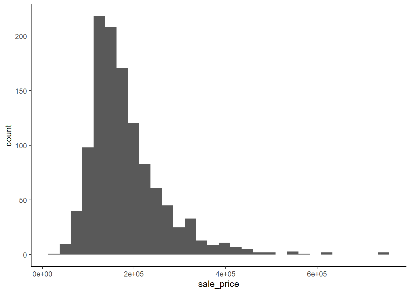
But you can also do quick plots in ggplot

\(summary()\) is useful too
##    Min. 1st Qu.  Median    Mean 3rd Qu.    Max.
##   34900  129925  163000  182404  214000  755000
and now lets start considering machine learning models…
2.2 The General Linear Model
We will start with a review of the use of the general linear model (GLM) as a machine learning model because you should be very familiar with this statistical model at this point
2.2.1 Simple Regression
We will start with simple linear regression with one predictor
\[Y = \beta_0 + \beta_1*X_1 + \epsilon\]
Applied to our regression problem, we might fit a model such as:
\[sale\_price = \beta_0 + \beta_1*gr\_liv\_area + \epsilon\]
We need to estimate \(\beta_0\) and \(\beta_1\) using our training dataset
You already know how to do this using \(lm()\) in base R. However, we will use \(train()\) from the caret package.
We use the caret package because:
- It provides a standard interface to hundreds of types of machine learning models with a consistent interface
- It provides very strong and easy pre-processing routines (e.g., missing data, scaling, transformations, near-zero variance, collinearity)
- It simplifies cross validation
- It supports numerous performance metrics
- It makes life easy
- …but we need to fully understand what it is doing b/c sometimes we need to do things outside of caret
We need to:
- Build a tibble with Y and all Xs (e.g., train_sr1)
- Set up a train control object that will be shared by many models
- Fit the model in the training dataset
train_sr1 <- select(train_all, sale_price, gr_liv_area)

trn_ctrl <- trainControl(method = "none")

sr1 <- train(sale_price ~ gr_liv_area, data = train_sr1,
            method = "glm", trControl = trn_ctrl)
\(train()\) returns a model object that contains a lot of information
You can begin to explore these on your own
##  [1] "method"       "modelInfo"    "modelType"    "results"      "pred"
##  [6] "bestTune"     "call"         "dots"         "metric"       "control"
## [11] "finalModel"   "preProcess"   "trainingData" "resample"     "resampledCM"
## [16] "perfNames"    "maximize"     "yLimits"      "times"        "levels"
## [21] "terms" "coefnames" "xlevels"## [1] "coefficients" "residuals" "fitted.values" "effects"
## [5] "R" "rank" "qr" "family"
## [9] "linear.predictors" "deviance" "aic" "null.deviance"
## [13] "iter" "weights" "prior.weights" "df.residual"
## [17] "df.null" "y" "converged" "boundary"
## [21] "model" "formula" "terms" "data"
## [25] "offset" "control" "method" "contrasts"
## [29] "xlevels" "xNames" "problemType" "tuneValue"
## [33] "obsLevels" "param"We can get the coefficients for this model using an extractor function
This is good generally practice in R
## (Intercept) gr_liv_area
##   9461.4933    113.8802
This indicates that our prediction model is: \[\hat{sale\_price} = 9461.5 + 113.9 * gr\_liv\_area\]
We can also get parameter estimates, standard errors and statistical tests for each \(\beta\) = 0 using \(summary()\)
##
## Call:
## NULL
##
## Deviance Residuals:
##     Min       1Q   Median       3Q      Max
## -357215   -29534     -561    22424   332983
##
## Coefficients:
##             Estimate Std. Error t value Pr(>|t|)
## (Intercept)  9461.49    5044.03   1.876   0.0609 .
## gr_liv_area   113.88       3.14  36.270   <2e-16 ***
## ---
## Signif. codes:  0 '***' 0.001 '**' 0.01 '*' 0.05 '.' 0.1 ' ' 1
##
## (Dispersion parameter for gaussian family taken to be 3167018547)
##
##     Null deviance: 7.8654e+12  on 1169  degrees of freedom
## Residual deviance: 3.6991e+12  on 1168  degrees of freedom
## AIC: 28919
##
## Number of Fisher Scoring iterations: 2
NOTE: We used the generalized linear model algorithm with default (gaussian) error term and default (linear) link function. Solved by maximum likelihood but statistically equivalent to the least squares solution.
We can get the \(\hat{sale\_price}\) in our training dataset using \(predict()\)
Here are the first 10 values for \(\hat{sale\_price}\):
##        1        2        3        4        5        6        7        8        9       10
## 204196.6 212851.5 164566.3 202374.5 211484.9 132110.4 127896.9 113320.2 152153.3 106715.2
How can we tell how well this model fits our training data?
- We could plot the prediction line over the raw data to visualize the fit (see below). To quantify the fit, we need a performance metric. Root mean square error would tell us the average size of the errors in the original units, dollars
What else do we really want to know?
- Training error is not that informative. We want to know about performance/errors for this model in new data such as the test dataset
Here is a plot of \(\hat{sale\_price}\) by \(gr\_liv\_area\) superimposed over a scatterplot of the raw data from the training dataset
ggplot(data = train_sr1, aes(x = gr_liv_area)) +
  geom_point(aes(y = sale_price), color = "gray") +
  geom_line(aes(y = predict(sr1)), size = 1.25, color = "blue") +
  ggtitle("Training")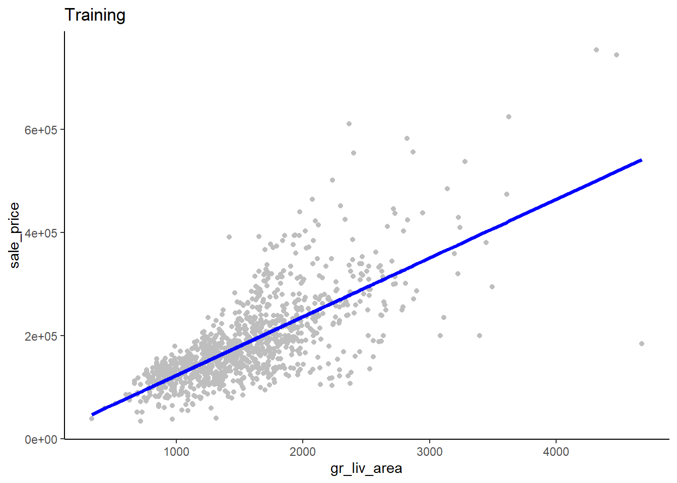
What do you notice in this plot, why might this be, and what might you consider doing?
- There is heteroscadasticity in the errors. The size of the errors increases for increasing predicted sale_price. We could transform (e.g., log) sale_price to correct this. In fact, Kaggle does this in their competition for this dataset and you will do this on the homework. For class, we will continue to use raw sale_price. Pros/Cons?
Here is code to calculate RMSE explicitly (for understanding) in our training dataset
rmse_demo <- tibble(sale_price = train_sr1$sale_price,
                     predicted = y_hat,
                     diff = sale_price - predicted,
                     diff_sqr = diff^2)
rmse_demo
## # A tibble: 1,170 x 4
## sale_price predicted diff diff_sqr
## <dbl> <dbl> <dbl> <dbl>
## 1 208500 204197. 4303. 18519487.
## 2 223500 212851. 10649. 113391297.
## 3 143000 164566. -21566. 465104250.
## 4 307000 202374. 104626. 10946497347.
## 5 129900 211485. -81585. 6656096405.
## 6 118000 132110. -14110. 199104212.
## 7 129500 127897. 1603. 2570048.
## 8 144000 113320. 30680. 941249991.
## 9 157000 152153. 4847. 23490133.
## 10 132000 106715. 25285. 639323500.
## # … with 1,160 more rows## [1] 56228.15However, you can use the \(RMSE()\) function in the caret package for this more easily
## [1] 56228.15We recognize that this model may be somewhat overfit to the training data set
Do you expect overfitting to be a big issue here? Why or why not?
- In this instance, there shouldnt be too much/any overfitting. The model (simple linear regression) is not very flexible, p is low (1 predictor), and the sample size is pretty large (N = 1460). This will very rarely be true in real modeling situations
Regardless, we care most about how this model will perform in new data
- Note that for new data we need to provide the new data to \(predict()\)
- Note use of \(kable()\) for simple tables in R Markdown
rmse_test_sr1 <- RMSE(predict(sr1, test), test$sale_price)

rmse <- bind_rows(rmse, tibble(model = "simple regression", rmse_train = rmse_train_sr1, rmse_test = rmse_test_sr1))
library(knitr)
kable(rmse)| model | rmse_train | rmse_test |
|---|---|---|
| simple regression | 56228.15 | 55871.92 |
The average error for our model’s predictions is about $56K. Not very good.
2.2.2 Extension to Multiple Linear Regression
We can improve model performance by moving from simple linear regression to multiple regression
##  [1] "ms_sub_class"    "ms_zoning"       "lot_frontage"    "lot_area"
##  [5] "street"          "alley"           "lot_shape"       "land_contour"
##  [9] "utilities"       "lot_config"      "land_slope"      "neighborhood"
## [13] "condition1"      "condition2"      "bldg_type"       "house_style"
## [17] "overall_qual"    "overall_cond"    "year_built"      "year_remod_add"
## [21] "roof_style"      "roof_matl"       "exterior1st"     "exterior2nd"
## [25] "mas_vnr_type"    "mas_vnr_area"    "exter_qual"      "exter_cond"
## [29] "foundation"      "bsmt_qual"       "bsmt_cond"       "bsmt_exposure"
## [33] "bsmt_fin_type1"  "bsmt_fin_sf1"    "bsmt_fin_type2"  "bsmt_fin_sf2"
## [37] "bsmt_unf_sf"     "total_bsmt_sf"   "heating"         "heating_qc"
## [41] "central_air"     "electrical"      "x1st_flr_sf"     "x2nd_flr_sf"
## [45] "low_qual_fin_sf" "gr_liv_area"     "bsmt_full_bath"  "bsmt_half_bath"
## [49] "full_bath"       "half_bath"       "bedroom_abv_gr"  "kitchen_abv_gr"
## [53] "kitchen_qual"    "tot_rms_abv_grd" "functional"      "fireplaces"
## [57] "fireplace_qu"    "garage_type"     "garage_yr_blt"   "garage_finish"
## [61] "garage_cars"     "garage_area"     "garage_qual"     "garage_cond"
## [65] "paved_drive"     "wood_deck_sf"    "open_porch_sf"   "enclosed_porch"
## [69] "x3ssn_porch"     "screen_porch"    "pool_area"       "pool_qc"
## [73] "fence"           "misc_feature"    "misc_val"        "mo_sold"
## [77] "yr_sold"         "sale_type"       "sale_condition"  "sale_price"
Lets expand our model to also include \(lot\_area\), \(year\_built\), \(overall\_qual\), and \(garage\_cars\)
Notes:
- Use of ‘.’ in the model formula in \(train()\)
- Use of earlier established trn_ctrl object
train_mr1 <- train_all %>%
  select(sale_price,
         gr_liv_area,
         lot_area,
         year_built,
         overall_qual,
         garage_cars)

mr1 <- train(sale_price ~ ., data = train_mr1,
            method = "glm", trControl = trn_ctrl)
This yields:
##   (Intercept)   gr_liv_area      lot_area    year_built  overall_qual   garage_cars
## -8.521196e+05  5.831055e+01  9.986847e-01  3.888901e+02  2.348331e+04  1.449096e+04
\[\hat{sale\_price} = -8.521196\times 10^{5} + 58.3 * gr\_liv\_area + 1 * lot\_area + 388.9 * year\_built + 2.34833\times 10^{4} * overall\_qual + 1.4491\times 10^{4} * garage\_cars\]
Compared with our previous simple regression model: \[\hat{sale\_price} = 9461.5 + 113.9 * gr\_liv\_area\]
What are the implications of the likely correlations among many of these predictors?
- The multiple regression model coefficients represent unique effects, controlling for all other variables in the model. You can see how the unique effect of gr_liv_area is smaller than its overall effect from the simple regression. This also means that the overall predictive strength of the model wont be a sum of the effects of each predictor considered in isolation - it will likely be less. Also, if the correlations are high, problems with multicollinearity will emerge. This will yield large standard errors which means that the models will start to have more variance when fit in different training datasets! We will soon learn about other regularized versions of the GLM that dont have these issues with correlated predictors.
Useful visualization of correlation matrix offered by \(corrplot()\)
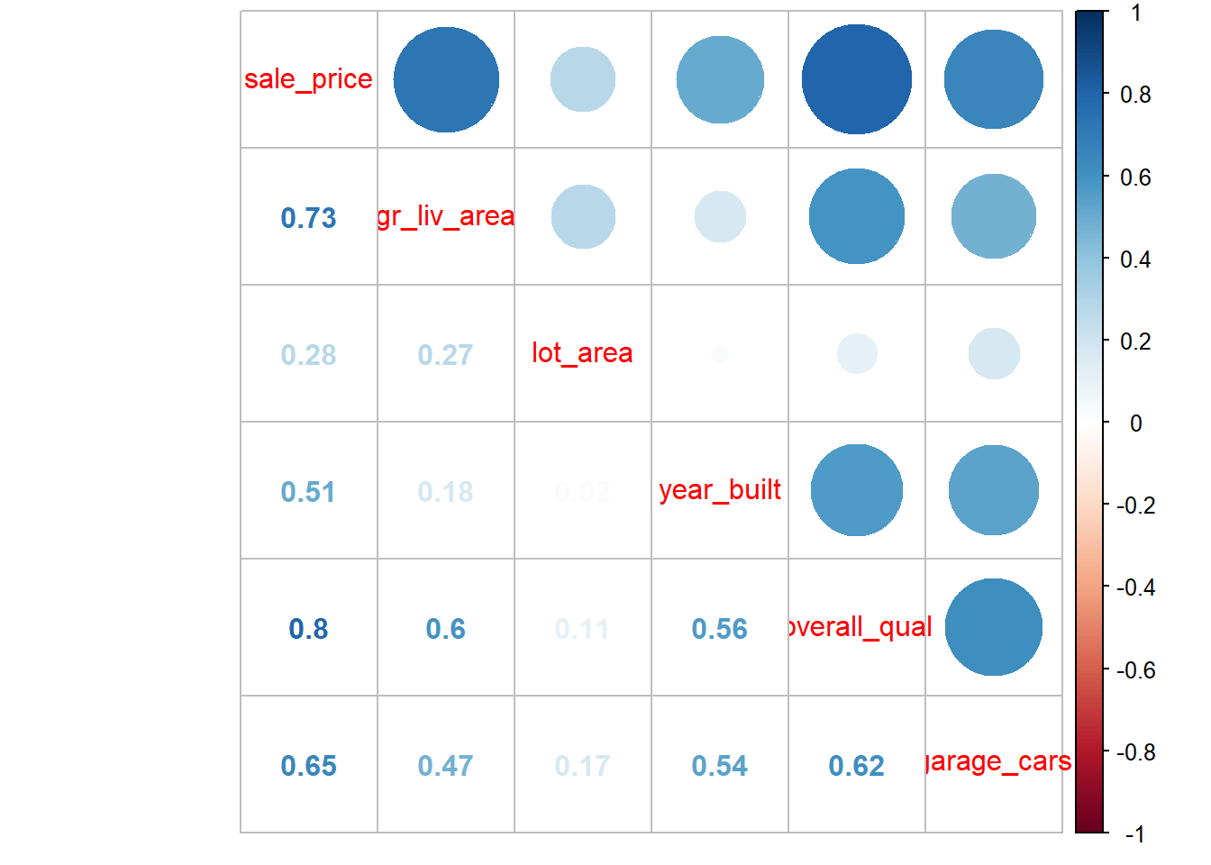
Of course, multicollinearity and SE inflation for any variable is based on its \(R^2\) using all other predictors
How well does this more complex model do in:
- training?
- and test?
rmse_train_mr1 <- RMSE(predict(mr1), train_mr1$sale_price)
rmse_test_mr1 <- RMSE(predict(mr1, test), test$sale_price)

rmse <- bind_rows(rmse, tibble(model = "multiple regression", rmse_train = rmse_train_mr1, rmse_test = rmse_test_mr1))
kable(rmse)| model | rmse_train | rmse_test |
|---|---|---|
| simple regression | 56228.15 | 55871.92 |
| multiple regression | 38663.97 | 40789.77 |
What are your observations about these performance results?
- First, you can also see that this still pretty simple multiple regression model is beginning to overfit the training data. You can tell this because its performance in test (average error = ~41K) is worse than in training (~ 39K). However, the more complex model is still definitely better at making predictions in new data (average prediction error of ~$41K vs. $56K). It seems to be a better model
2.2.3 Extension to Categorical Predictors
Many important predictors in our models may be categorical (i.e., nominal) rather than quantitative (e.g., ordinal, interval, ratio)
How do you handle categorical predictors in linear regression?
- We use a categorical coding scheme such as dummy codes, contrast codes, etc. This yields multiple ‘regressors’ (or features) for each categorical predictor. Specifically, an m level categorical predictor resulted in m-1 regressors
For example, with dummy coding:
| Race | Race1 | Race2 |
|---|---|---|
| Black | 1 | 0 |
| White | 0 | 1 |
| Other | 0 | 0 |
Notes:
- Any full rank (m-1) set of regressors regardless of coding system predicts exactly the same
- Preference among coding systems is simply to get single df contrasts of theoretical importance
- Final (mth) regressor is not included b/c its is completely redundant (perfectly multicollinear) with other regressors. This would also prevent the model from fitting (‘dummy variable trap’).
Lets consider some potentially important categorical predictors for our model
##
## C (all)      FV      RH      RL      RM
## 8 57 12 913 180##
## Corner CulDSac FR2 FR3 Inside
## 212 78 34 4 842##
## 1Fam 2fmCon Duplex Twnhs TwnhsE
## 981 24 43 34 88There are many ways to code dummy variables in R. We focus on two:
- Using \(factor()\) and \(contrasts()\) from base R
- Using \(dummyVars()\) from caret package
For both methods, we will calculate the dummy codes in the full data and then re-split into train/test (Why?)
You can use \(factor()\) and \(contrasts()\) from base R to set contrasts for specific variables
This converts character variables to factors and sets contrasts
It does NOT add the dummy predictors directly to the tibble. R handles that internally.
- Good for including interactions with these factors
- Need to consider how missing data is handled?
ames <- ames %>%
  mutate(ms_zoning = factor(ms_zoning),
         lot_config = factor(lot_config),
         bldg_type = factor(bldg_type))
contrasts(ames$ms_zoning) <- contr.treatment(length(levels(ames$ms_zoning)))
contrasts(ames$lot_config) <- contr.treatment(length(levels(ames$lot_config)))
contrasts(ames$bldg_type) <- contr.treatment(length(levels(ames$bldg_type)))

names(ames)
## [1] "ms_sub_class" "ms_zoning" "lot_frontage" "lot_area"
## [5] "street" "alley" "lot_shape" "land_contour"
## [9] "utilities" "lot_config" "land_slope" "neighborhood"
## [13] "condition1" "condition2" "bldg_type" "house_style"
## [17] "overall_qual" "overall_cond" "year_built" "year_remod_add"
## [21] "roof_style" "roof_matl" "exterior1st" "exterior2nd"
## [25] "mas_vnr_type" "mas_vnr_area" "exter_qual" "exter_cond"
## [29] "foundation" "bsmt_qual" "bsmt_cond" "bsmt_exposure"
## [33] "bsmt_fin_type1" "bsmt_fin_sf1" "bsmt_fin_type2" "bsmt_fin_sf2"
## [37] "bsmt_unf_sf" "total_bsmt_sf" "heating" "heating_qc"
## [41] "central_air" "electrical" "x1st_flr_sf" "x2nd_flr_sf"
## [45] "low_qual_fin_sf" "gr_liv_area" "bsmt_full_bath" "bsmt_half_bath"
## [49] "full_bath" "half_bath" "bedroom_abv_gr" "kitchen_abv_gr"
## [53] "kitchen_qual" "tot_rms_abv_grd" "functional" "fireplaces"
## [57] "fireplace_qu" "garage_type" "garage_yr_blt" "garage_finish"
## [61] "garage_cars" "garage_area" "garage_qual" "garage_cond"
## [65] "paved_drive" "wood_deck_sf" "open_porch_sf" "enclosed_porch"
## [69] "x3ssn_porch" "screen_porch" "pool_area" "pool_qc"
## [73] "fence" "misc_feature" "misc_val" "mo_sold"
## [77] "yr_sold" "sale_type" "sale_condition" "sale_price"## 2 3 4 5
## C (all) 0 0 0 0
## FV 1 0 0 0
## RH 0 1 0 0
## RL 0 0 1 0
## RM 0 0 0 1You can also do all character and factor variables at once by using \(mutate\_if()\) and setting appropriate contrasts in \(options()\)
Note that this will override any factor contrasts you have set and change your default contrast options. Adjust accordingly.
options(contrasts=c('contr.treatment','contr.poly'))
ames <- ames %>%
  mutate_if(is.factor, as.character) %>%
  mutate_if(is.character, as.factor)
You can use \(dummyVars()\) from caret to create explicit dummy code variables:
- Note use of \(fullRank = TRUE\) (not default) to get true dummy codes (vs. one-hot codes)
- Can use with character or factor variables
- This will create new columns in the tibble for the dummy variables
- This also retains original character variable in the tibble (modify as needed)
- BUG REPORT: \(sep\) does not currently work with character variables. May want to change to factor first to retain snake case variable names.
ames <- read_csv(file.path(data_path, "ames.csv")) %>%
  clean_names(case = "snake") %>%
  select(-id) %>%
  mutate_if(is.character, as.factor) #to address variable name bug in dummyVars()

dmy_codes <- dummyVars(~ ms_zoning + lot_config + bldg_type, fullRank = TRUE, sep = "_", data = ames)

ames <- ames %>%
  bind_cols(as_tibble(predict(dmy_codes, ames))) %>%
  glimpse()
## Observations: 1,460
## Variables: 92
## $ ms_sub_class <dbl> 60, 20, 60, 70, 60, 50, 20, 60, 50, 190, 20, 60, 20, 20, 20, …
## $ ms_zoning <fct> RL, RL, RL, RL, RL, RL, RL, RL, RM, RL, RL, RL, RL, RL, RL, R…
## $ lot_frontage <dbl> 65, 80, 68, 60, 84, 85, 75, NA, 51, 50, 70, 85, NA, 91, NA, 5…
## $ lot_area <dbl> 8450, 9600, 11250, 9550, 14260, 14115, 10084, 10382, 6120, 74…
## $ street <fct> Pave, Pave, Pave, Pave, Pave, Pave, Pave, Pave, Pave, Pave, P…
## $ alley <fct> NA, NA, NA, NA, NA, NA, NA, NA, NA, NA, NA, NA, NA, NA, NA, N…
## $ lot_shape <fct> Reg, Reg, IR1, IR1, IR1, IR1, Reg, IR1, Reg, Reg, Reg, IR1, I…
## $ land_contour <fct> Lvl, Lvl, Lvl, Lvl, Lvl, Lvl, Lvl, Lvl, Lvl, Lvl, Lvl, Lvl, L…
## $ utilities <fct> AllPub, AllPub, AllPub, AllPub, AllPub, AllPub, AllPub, AllPu…
## $ lot_config <fct> Inside, FR2, Inside, Corner, FR2, Inside, Inside, Corner, Ins…
## $ land_slope <fct> Gtl, Gtl, Gtl, Gtl, Gtl, Gtl, Gtl, Gtl, Gtl, Gtl, Gtl, Gtl, G…
## $ neighborhood <fct> CollgCr, Veenker, CollgCr, Crawfor, NoRidge, Mitchel, Somerst…
## $ condition1 <fct> Norm, Feedr, Norm, Norm, Norm, Norm, Norm, PosN, Artery, Arte…
## $ condition2 <fct> Norm, Norm, Norm, Norm, Norm, Norm, Norm, Norm, Norm, Artery,…
## $ bldg_type <fct> 1Fam, 1Fam, 1Fam, 1Fam, 1Fam, 1Fam, 1Fam, 1Fam, 1Fam, 2fmCon,…
## $ house_style <fct> 2Story, 1Story, 2Story, 2Story, 2Story, 1.5Fin, 1Story, 2Stor…
## $ overall_qual <dbl> 7, 6, 7, 7, 8, 5, 8, 7, 7, 5, 5, 9, 5, 7, 6, 7, 6, 4, 5, 5, 8…
## $ overall_cond <dbl> 5, 8, 5, 5, 5, 5, 5, 6, 5, 6, 5, 5, 6, 5, 5, 8, 7, 5, 5, 6, 5…
## $ year_built <dbl> 2003, 1976, 2001, 1915, 2000, 1993, 2004, 1973, 1931, 1939, 1…
## $ year_remod_add <dbl> 2003, 1976, 2002, 1970, 2000, 1995, 2005, 1973, 1950, 1950, 1…
## $ roof_style <fct> Gable, Gable, Gable, Gable, Gable, Gable, Gable, Gable, Gable…
## $ roof_matl <fct> CompShg, CompShg, CompShg, CompShg, CompShg, CompShg, CompShg…
## $ exterior1st <fct> VinylSd, MetalSd, VinylSd, Wd Sdng, VinylSd, VinylSd, VinylSd…
## $ exterior2nd <fct> VinylSd, MetalSd, VinylSd, Wd Shng, VinylSd, VinylSd, VinylSd…
## $ mas_vnr_type <fct> BrkFace, None, BrkFace, None, BrkFace, None, Stone, Stone, No…
## $ mas_vnr_area <dbl> 196, 0, 162, 0, 350, 0, 186, 240, 0, 0, 0, 286, 0, 306, 212, …
## $ exter_qual <fct> Gd, TA, Gd, TA, Gd, TA, Gd, TA, TA, TA, TA, Ex, TA, Gd, TA, T…
## $ exter_cond <fct> TA, TA, TA, TA, TA, TA, TA, TA, TA, TA, TA, TA, TA, TA, TA, T…
## $ foundation <fct> PConc, CBlock, PConc, BrkTil, PConc, Wood, PConc, CBlock, Brk…
## $ bsmt_qual <fct> Gd, Gd, Gd, TA, Gd, Gd, Ex, Gd, TA, TA, TA, Ex, TA, Gd, TA, T…
## $ bsmt_cond <fct> TA, TA, TA, Gd, TA, TA, TA, TA, TA, TA, TA, TA, TA, TA, TA, T…
## $ bsmt_exposure <fct> No, Gd, Mn, No, Av, No, Av, Mn, No, No, No, No, No, Av, No, N…
## $ bsmt_fin_type1 <fct> GLQ, ALQ, GLQ, ALQ, GLQ, GLQ, GLQ, ALQ, Unf, GLQ, Rec, GLQ, A…
## $ bsmt_fin_sf1 <dbl> 706, 978, 486, 216, 655, 732, 1369, 859, 0, 851, 906, 998, 73…
## $ bsmt_fin_type2 <fct> Unf, Unf, Unf, Unf, Unf, Unf, Unf, BLQ, Unf, Unf, Unf, Unf, U…
## $ bsmt_fin_sf2 <dbl> 0, 0, 0, 0, 0, 0, 0, 32, 0, 0, 0, 0, 0, 0, 0, 0, 0, 0, 0, 0, …
## $ bsmt_unf_sf <dbl> 150, 284, 434, 540, 490, 64, 317, 216, 952, 140, 134, 177, 17…
## $ total_bsmt_sf <dbl> 856, 1262, 920, 756, 1145, 796, 1686, 1107, 952, 991, 1040, 1…
## $ heating <fct> GasA, GasA, GasA, GasA, GasA, GasA, GasA, GasA, GasA, GasA, G…
## $ heating_qc <fct> Ex, Ex, Ex, Gd, Ex, Ex, Ex, Ex, Gd, Ex, Ex, Ex, TA, Ex, TA, E…
## $ central_air <fct> Y, Y, Y, Y, Y, Y, Y, Y, Y, Y, Y, Y, Y, Y, Y, Y, Y, Y, Y, Y, Y…
## $ electrical <fct> SBrkr, SBrkr, SBrkr, SBrkr, SBrkr, SBrkr, SBrkr, SBrkr, FuseF…
## $ x1st_flr_sf <dbl> 856, 1262, 920, 961, 1145, 796, 1694, 1107, 1022, 1077, 1040,…
## $ x2nd_flr_sf <dbl> 854, 0, 866, 756, 1053, 566, 0, 983, 752, 0, 0, 1142, 0, 0, 0…
## $ low_qual_fin_sf <dbl> 0, 0, 0, 0, 0, 0, 0, 0, 0, 0, 0, 0, 0, 0, 0, 0, 0, 0, 0, 0, 0…
## $ gr_liv_area <dbl> 1710, 1262, 1786, 1717, 2198, 1362, 1694, 2090, 1774, 1077, 1…
## $ bsmt_full_bath <dbl> 1, 0, 1, 1, 1, 1, 1, 1, 0, 1, 1, 1, 1, 0, 1, 0, 1, 0, 1, 0, 0…
## $ bsmt_half_bath <dbl> 0, 1, 0, 0, 0, 0, 0, 0, 0, 0, 0, 0, 0, 0, 0, 0, 0, 0, 0, 0, 0…
## $ full_bath <dbl> 2, 2, 2, 1, 2, 1, 2, 2, 2, 1, 1, 3, 1, 2, 1, 1, 1, 2, 1, 1, 3…
## $ half_bath <dbl> 1, 0, 1, 0, 1, 1, 0, 1, 0, 0, 0, 0, 0, 0, 1, 0, 0, 0, 1, 0, 1…
## $ bedroom_abv_gr <dbl> 3, 3, 3, 3, 4, 1, 3, 3, 2, 2, 3, 4, 2, 3, 2, 2, 2, 2, 3, 3, 4…
## $ kitchen_abv_gr <dbl> 1, 1, 1, 1, 1, 1, 1, 1, 2, 2, 1, 1, 1, 1, 1, 1, 1, 2, 1, 1, 1…
## $ kitchen_qual <fct> Gd, TA, Gd, Gd, Gd, TA, Gd, TA, TA, TA, TA, Ex, TA, Gd, TA, T…
## $ tot_rms_abv_grd <dbl> 8, 6, 6, 7, 9, 5, 7, 7, 8, 5, 5, 11, 4, 7, 5, 5, 5, 6, 6, 6, …
## $ functional <fct> Typ, Typ, Typ, Typ, Typ, Typ, Typ, Typ, Min1, Typ, Typ, Typ, …
## $ fireplaces <dbl> 0, 1, 1, 1, 1, 0, 1, 2, 2, 2, 0, 2, 0, 1, 1, 0, 1, 0, 0, 0, 1…
## $ fireplace_qu <fct> NA, TA, TA, Gd, TA, NA, Gd, TA, TA, TA, NA, Gd, NA, Gd, Fa, N…
## $ garage_type <fct> Attchd, Attchd, Attchd, Detchd, Attchd, Attchd, Attchd, Attch…
## $ garage_yr_blt <dbl> 2003, 1976, 2001, 1998, 2000, 1993, 2004, 1973, 1931, 1939, 1…
## $ garage_finish <fct> RFn, RFn, RFn, Unf, RFn, Unf, RFn, RFn, Unf, RFn, Unf, Fin, U…
## $ garage_cars <dbl> 2, 2, 2, 3, 3, 2, 2, 2, 2, 1, 1, 3, 1, 3, 1, 2, 2, 2, 2, 1, 3…
## $ garage_area <dbl> 548, 460, 608, 642, 836, 480, 636, 484, 468, 205, 384, 736, 3…
## $ garage_qual <fct> TA, TA, TA, TA, TA, TA, TA, TA, Fa, Gd, TA, TA, TA, TA, TA, T…
## $ garage_cond <fct> TA, TA, TA, TA, TA, TA, TA, TA, TA, TA, TA, TA, TA, TA, TA, T…
## $ paved_drive <fct> Y, Y, Y, Y, Y, Y, Y, Y, Y, Y, Y, Y, Y, Y, Y, Y, Y, Y, Y, Y, Y…
## $ wood_deck_sf <dbl> 0, 298, 0, 0, 192, 40, 255, 235, 90, 0, 0, 147, 140, 160, 0, …
## $ open_porch_sf <dbl> 61, 0, 42, 35, 84, 30, 57, 204, 0, 4, 0, 21, 0, 33, 213, 112,…
## $ enclosed_porch <dbl> 0, 0, 0, 272, 0, 0, 0, 228, 205, 0, 0, 0, 0, 0, 176, 0, 0, 0,…
## $ x3ssn_porch <dbl> 0, 0, 0, 0, 0, 320, 0, 0, 0, 0, 0, 0, 0, 0, 0, 0, 0, 0, 0, 0,…
## $ screen_porch <dbl> 0, 0, 0, 0, 0, 0, 0, 0, 0, 0, 0, 0, 176, 0, 0, 0, 0, 0, 0, 0,…
## $ pool_area <dbl> 0, 0, 0, 0, 0, 0, 0, 0, 0, 0, 0, 0, 0, 0, 0, 0, 0, 0, 0, 0, 0…
## $ pool_qc <fct> NA, NA, NA, NA, NA, NA, NA, NA, NA, NA, NA, NA, NA, NA, NA, N…
## $ fence <fct> NA, NA, NA, NA, NA, MnPrv, NA, NA, NA, NA, NA, NA, NA, NA, Gd…
## $ misc_feature <fct> NA, NA, NA, NA, NA, Shed, NA, Shed, NA, NA, NA, NA, NA, NA, N…
## $ misc_val <dbl> 0, 0, 0, 0, 0, 700, 0, 350, 0, 0, 0, 0, 0, 0, 0, 0, 700, 500,…
## $ mo_sold <dbl> 2, 5, 9, 2, 12, 10, 8, 11, 4, 1, 2, 7, 9, 8, 5, 7, 3, 10, 6, …
## $ yr_sold <dbl> 2008, 2007, 2008, 2006, 2008, 2009, 2007, 2009, 2008, 2008, 2…
## $ sale_type <fct> WD, WD, WD, WD, WD, WD, WD, WD, WD, WD, WD, New, WD, New, WD,…
## $ sale_condition <fct> Normal, Normal, Normal, Abnorml, Normal, Normal, Normal, Norm…
## $ sale_price <dbl> 208500, 181500, 223500, 140000, 250000, 143000, 307000, 20000…
## $ ms_zoning_FV <dbl> 0, 0, 0, 0, 0, 0, 0, 0, 0, 0, 0, 0, 0, 0, 0, 0, 0, 0, 0, 0, 0…
## $ ms_zoning_RH <dbl> 0, 0, 0, 0, 0, 0, 0, 0, 0, 0, 0, 0, 0, 0, 0, 0, 0, 0, 0, 0, 0…
## $ ms_zoning_RL <dbl> 1, 1, 1, 1, 1, 1, 1, 1, 0, 1, 1, 1, 1, 1, 1, 0, 1, 1, 1, 1, 1…
## $ ms_zoning_RM <dbl> 0, 0, 0, 0, 0, 0, 0, 0, 1, 0, 0, 0, 0, 0, 0, 1, 0, 0, 0, 0, 0…
## $ lot_config_CulDSac <dbl> 0, 0, 0, 0, 0, 0, 0, 0, 0, 0, 0, 0, 0, 0, 0, 0, 1, 0, 0, 0, 0…
## $ lot_config_FR2 <dbl> 0, 1, 0, 0, 1, 0, 0, 0, 0, 0, 0, 0, 0, 0, 0, 0, 0, 0, 0, 0, 0…
## $ lot_config_FR3 <dbl> 0, 0, 0, 0, 0, 0, 0, 0, 0, 0, 0, 0, 0, 0, 0, 0, 0, 0, 0, 0, 0…
## $ lot_config_Inside <dbl> 1, 0, 1, 0, 0, 1, 1, 0, 1, 0, 1, 1, 1, 1, 0, 0, 0, 1, 1, 1, 0…
## $ bldg_type_2fmCon <dbl> 0, 0, 0, 0, 0, 0, 0, 0, 0, 1, 0, 0, 0, 0, 0, 0, 0, 0, 0, 0, 0…
## $ bldg_type_Duplex <dbl> 0, 0, 0, 0, 0, 0, 0, 0, 0, 0, 0, 0, 0, 0, 0, 0, 0, 1, 0, 0, 0…
## $ bldg_type_Twnhs <dbl> 0, 0, 0, 0, 0, 0, 0, 0, 0, 0, 0, 0, 0, 0, 0, 0, 0, 0, 0, 0, 0…
## $ bldg_type_TwnhsE <dbl> 0, 0, 0, 0, 0, 0, 0, 0, 0, 0, 0, 0, 0, 0, 0, 0, 0, 0, 0, 0, 0…You can use \(dummyVars()\) for one-hot codes as well:
One-hot codes are less than full rank. They include one new dummy variable for EVERY level of the categorical variable.
Each dummy variable is coded 1 for its target level and zero for all other levels
For example, with one-hot coding:
| Race | Race1 | Race2 | Race3 |
|---|---|---|---|
| Black | 1 | 0 | 0 |
| White | 0 | 1 | 0 |
| Other | 0 | 0 | 1 |
- This set will not work with types of models that dont regularize in some manner
- Dont use with lm, glm models
- Can (and should?) use with lasso, ridge, glmnet, svm models (more on these later)
- Coefficients are not interpretable as the contrast of target vs. reference. (Instead, its simply target vs. all other controlling for all other variables?)
Notes:
- Note use of \(drop2nd = TRUE\)
- Note use of ‘~ .’ to code all factor and character variables at the same time. Ignores quantitative variables. Be careful.
dmy_codes <- dummyVars(~ ., fullRank = FALSE, drop2nd = TRUE, data = ames)

ames <- ames %>%
  bind_cols(as_tibble(predict(dmy_codes, ames))) %>%
  glimpse()
Regardless of the method (using \(dummyVars()\) method here), we follow with a re-split into train/test and make subset of train for model fitting
Note use of same seed as before
set.seed(19690127)
ames_splits <- initial_split(ames, prop = .8, strata = "sale_price")
train_all <- training(ames_splits)
test <- testing(ames_splits)

train_mr2 <- train_all %>%
  select(sale_price,
         gr_liv_area,
         lot_area,
         year_built,
         overall_qual,
         garage_cars,
         starts_with("ms_zoning"),
         starts_with("lot_config"),
         starts_with("bldg_type")) %>%
  select(-ms_zoning, -lot_config, -bldg_type) %>%
  glimpse()
## Observations: 1,170
## Variables: 18
## $ sale_price <dbl> 208500, 223500, 143000, 307000, 129900, 118000, 129500, 14400…
## $ gr_liv_area <dbl> 1710, 1786, 1362, 1694, 1774, 1077, 1040, 912, 1253, 854, 129…
## $ lot_area <dbl> 8450, 11250, 14115, 10084, 6120, 7420, 11200, 12968, 10920, 6…
## $ year_built <dbl> 2003, 2001, 1993, 2004, 1931, 1939, 1965, 1962, 1960, 1929, 1…
## $ overall_qual <dbl> 7, 7, 5, 8, 7, 5, 5, 5, 6, 7, 4, 5, 5, 8, 7, 8, 5, 5, 8, 5, 8…
## $ garage_cars <dbl> 2, 2, 2, 2, 2, 1, 1, 1, 1, 2, 2, 2, 1, 3, 1, 2, 2, 1, 3, 2, 3…
## $ ms_zoning_FV <dbl> 0, 0, 0, 0, 0, 0, 0, 0, 0, 0, 0, 0, 0, 0, 0, 0, 0, 0, 0, 0, 0…
## $ ms_zoning_RH <dbl> 0, 0, 0, 0, 0, 0, 0, 0, 0, 0, 0, 0, 0, 0, 0, 0, 0, 0, 0, 0, 0…
## $ ms_zoning_RL <dbl> 1, 1, 1, 1, 0, 1, 1, 1, 1, 0, 1, 1, 1, 1, 0, 1, 0, 1, 1, 1, 1…
## $ ms_zoning_RM <dbl> 0, 0, 0, 0, 1, 0, 0, 0, 0, 1, 0, 0, 0, 0, 1, 0, 1, 0, 0, 0, 0…
## $ lot_config_CulDSac <dbl> 0, 0, 0, 0, 0, 0, 0, 0, 0, 0, 0, 0, 0, 0, 0, 0, 0, 0, 0, 0, 0…
## $ lot_config_FR2 <dbl> 0, 0, 0, 0, 0, 0, 0, 0, 0, 0, 0, 0, 0, 0, 0, 0, 0, 0, 0, 0, 0…
## $ lot_config_FR3 <dbl> 0, 0, 0, 0, 0, 0, 0, 0, 0, 0, 0, 0, 0, 0, 0, 0, 0, 0, 0, 0, 0…
## $ lot_config_Inside <dbl> 1, 1, 1, 1, 1, 0, 1, 1, 0, 0, 1, 1, 1, 0, 1, 1, 1, 1, 0, 0, 1…
## $ bldg_type_2fmCon <dbl> 0, 0, 0, 0, 0, 1, 0, 0, 0, 0, 0, 0, 0, 0, 0, 0, 0, 0, 0, 0, 0…
## $ bldg_type_Duplex <dbl> 0, 0, 0, 0, 0, 0, 0, 0, 0, 0, 1, 0, 0, 0, 0, 0, 0, 0, 0, 0, 0…
## $ bldg_type_Twnhs <dbl> 0, 0, 0, 0, 0, 0, 0, 0, 0, 0, 0, 0, 0, 0, 0, 0, 0, 0, 0, 0, 0…
## $ bldg_type_TwnhsE <dbl> 0, 0, 0, 0, 0, 0, 0, 0, 0, 0, 0, 0, 0, 0, 0, 0, 1, 0, 0, 0, 0…Fit the model in training set
Evaluate the model in:
- training
- test
mr2 <- train(sale_price ~ ., data = train_mr2,
            method = "glm", trControl = trn_ctrl)


rmse_train_mr2 <- RMSE(predict(mr2), train_mr2$sale_price)
rmse_test_mr2 <- RMSE(predict(mr2, test), test$sale_price)

rmse <- bind_rows(rmse, tibble(model = "multiple regression w/categorical", rmse_train = rmse_train_mr2, rmse_test = rmse_test_mr2))
kable(rmse)| model | rmse_train | rmse_test |
|---|---|---|
| simple regression | 56228.15 | 55871.92 |
| multiple regression | 38663.97 | 40789.77 |
| multiple regression w/categorical | 37700.56 | 39958.26 |
2.2.4 Extension to Interactive Models
There may be interactive effects among our predictors. These are easy to model as well.
For example, it may be that the relationship between \(year\_built\) and \(sale\_price\) depends on \(overall\_qual\). Lets include that in our model.
You can manually code interactions (as product terms) into the training and test
- Review the training and test error for our various incremental models below
- This interaction doesnt help
train_mr3 <- train_mr2 %>%
  mutate(year_built_X_overall_qual = year_built * overall_qual)
test <- test %>%
  mutate(year_built_X_overall_qual = year_built * overall_qual)

mr3_int1 <- train(sale_price ~ ., data = train_mr3,
            method = "glm", trControl = trn_ctrl)

rmse_train_mr3_int1 <- RMSE(predict(mr3_int1), train_mr3$sale_price)
rmse_test_mr3_int1 <- RMSE(predict(mr3_int1, test), test$sale_price)

rmse <- bind_rows(rmse, tibble(model = "multiple regression w/focal interaction", rmse_train = rmse_train_mr3_int1, rmse_test = rmse_test_mr3_int1))
kable(rmse)| model | rmse_train | rmse_test |
|---|---|---|
| simple regression | 56228.15 | 55871.92 |
| multiple regression | 38663.97 | 40789.77 |
| multiple regression w/categorical | 37700.56 | 39958.26 |
| multiple regression w/focal interaction | 36060.21 | 40673.83 |
Alternatively, you can include interactions as part of the formula in \(train()\)
Note that \(predict()\) needs to have training data explicitly provided. It has problems with \(year\_built:overall\_qual\) otherwise.
Comparison below shows the same result for the two methods for coding interactions on training error
train_mr3 <- train_mr3 %>%
  select(-year_built_X_overall_qual)

mr3_int2 <- train(sale_price ~ . + year_built:overall_qual, data = train_mr3,
            method = "glm", trControl = trn_ctrl)

RMSE(predict(mr3_int1), train_mr3$sale_price)
## [1] 36060.21## [1] 36060.21You can also code all interactions by formula.
- Easy if you have only quantitative variables
- Lets use train_mr1 (no categorical variables)
- This produces a sizable reduction in our estimate of test error
mr3_int3 <- train(sale_price ~ .^2, data = train_mr1,
            method = "glm", trControl = trn_ctrl)

coef(mr3_int3$finalModel)
## (Intercept) gr_liv_area lot_area
## 1.718428e+05 -1.212108e+02 2.000489e+01
## year_built overall_qual garage_cars
## -2.235404e+01 -1.852575e+05 8.716401e+04
## `gr_liv_area:lot_area` `gr_liv_area:year_built` `gr_liv_area:overall_qual`
## -2.643298e-03 4.959769e-02 1.595986e+01
## `gr_liv_area:garage_cars` `lot_area:year_built` `lot_area:overall_qual`
## 1.668575e+00 -8.768245e-03 2.640634e-01
## `lot_area:garage_cars` `year_built:overall_qual` `year_built:garage_cars`
## 8.062370e-01 8.575310e+01 -6.184345e+01
## `overall_qual:garage_cars`
## 6.425294e+03rmse_train_mr3_int3 <- RMSE(predict(mr3_int3, train_mr1), train_mr1$sale_price)
rmse_test_mr3_int3 <- RMSE(predict(mr3_int3, test), test$sale_price)
rmse <- bind_rows(rmse, tibble(model = "multiple regression w/all quant interactions", rmse_train = rmse_train_mr3_int3, rmse_test = rmse_test_mr3_int3))
kable(rmse)| model | rmse_train | rmse_test |
|---|---|---|
| simple regression | 56228.15 | 55871.92 |
| multiple regression | 38663.97 | 40789.77 |
| multiple regression w/categorical | 37700.56 | 39958.26 |
| multiple regression w/focal interaction | 36060.21 | 40673.83 |
| multiple regression w/all quant interactions | 32212.91 | 31747.06 |
You can also do this with categorical variables in the model
Below, we demonstrate this using train_mr2
This method requires that you have contrasts coded for the categorical interactions rather than explicit dummy variables (Why?)
This will often not work well if there are many empty cells among crossings of categorical variables
- Note the NAs for many coefficients of categorical interaction terms
mr3_int4 <- train(sale_price ~ .^2, data = train_mr3_contrasts,
            method = "glm", trControl = trn_ctrl)

coef(mr3_int4$finalModel)
## (Intercept) gr_liv_area lot_area
## 3.931392e+06 1.493084e+02 3.485288e+01
## year_built overall_qual garage_cars
## -2.033793e+03 -6.889771e+04 -1.539193e+04
## ms_zoning2 ms_zoning3 ms_zoning4
## -1.009947e+07 -5.139194e+06 -4.460264e+06
## ms_zoning5 lot_config2 lot_config3
## -4.961807e+06 -6.335447e+05 3.367930e+05
## lot_config4 lot_config5 bldg_type2
## 5.324519e+05 1.166233e+05 -1.957636e+05
## bldg_type3 bldg_type4 bldg_type5
## -9.585297e+05 3.541480e+06 -1.439545e+05
## `gr_liv_area:lot_area` `gr_liv_area:year_built` `gr_liv_area:overall_qual`
## -3.046236e-03 -1.396808e-01 1.780928e+01
## `gr_liv_area:garage_cars` `gr_liv_area:ms_zoning2` `gr_liv_area:ms_zoning3`
## 8.740158e-01 1.348914e+02 1.623326e+02
## `gr_liv_area:ms_zoning4` `gr_liv_area:ms_zoning5` `gr_liv_area:lot_config2`
## 1.084375e+02 8.779207e+01 2.036762e+01
## `gr_liv_area:lot_config3` `gr_liv_area:lot_config4` `gr_liv_area:lot_config5`
## 2.816908e+00 7.813031e+01 -1.627033e+01
## `gr_liv_area:bldg_type2` `gr_liv_area:bldg_type3` `gr_liv_area:bldg_type4`
## 1.662099e+01 3.844298e+00 4.711557e+00
## `gr_liv_area:bldg_type5` `lot_area:year_built` `lot_area:overall_qual`
## 2.398514e+01 -1.792369e-03 -2.064597e-01
## `lot_area:garage_cars` `lot_area:ms_zoning2` `lot_area:ms_zoning3`
## 1.799965e+00 -2.973522e+01 -2.851961e+01
## `lot_area:ms_zoning4` `lot_area:ms_zoning5` `lot_area:lot_config2`
## -2.684801e+01 -2.571080e+01 2.004276e-01
## `lot_area:lot_config3` `lot_area:lot_config4` `lot_area:lot_config5`
## -4.631749e-01 -5.649315e+00 -8.790018e-01
## `lot_area:bldg_type2` `lot_area:bldg_type3` `lot_area:bldg_type4`
## -1.230888e+00 1.565751e-01 2.872090e+01
## `lot_area:bldg_type5` `year_built:overall_qual` `year_built:garage_cars`
## 6.598574e+00 2.303124e+01 3.259434e+00
## `year_built:ms_zoning2` `year_built:ms_zoning3` `year_built:ms_zoning4`
## 5.258187e+03 2.721924e+03 2.375213e+03
## `year_built:ms_zoning5` `year_built:lot_config2` `year_built:lot_config3`
## 2.653688e+03 3.131233e+02 -1.823959e+02
## `year_built:lot_config4` `year_built:lot_config5` `year_built:bldg_type2`
## -3.126781e+02 -1.062299e+02 8.845717e+01
## `year_built:bldg_type3` `year_built:bldg_type4` `year_built:bldg_type5`
## 5.223817e+02 -1.829233e+03 3.769830e+01
## `overall_qual:garage_cars` `overall_qual:ms_zoning2` `overall_qual:ms_zoning3`
## 7.828153e+03 -1.259093e+04 -7.779410e+03
## `overall_qual:ms_zoning4` `overall_qual:ms_zoning5` `overall_qual:lot_config2`
## 3.327673e+03 -4.206880e+03 1.403645e+03
## `overall_qual:lot_config3` `overall_qual:lot_config4` `overall_qual:lot_config5`
## -1.180189e+03 NA 5.919450e+03
## `overall_qual:bldg_type2` `overall_qual:bldg_type3` `overall_qual:bldg_type4`
## -2.886776e+03 -1.423911e+04 -1.682317e+03
## `overall_qual:bldg_type5` `garage_cars:ms_zoning2` `garage_cars:ms_zoning3`
## 5.408636e+03 -5.820519e+04 -2.515368e+04
## `garage_cars:ms_zoning4` `garage_cars:ms_zoning5` `garage_cars:lot_config2`
## -4.240034e+04 -3.378025e+04 -1.206981e+04
## `garage_cars:lot_config3` `garage_cars:lot_config4` `garage_cars:lot_config5`
## 1.060910e+04 NA 2.998137e+03
## `garage_cars:bldg_type2` `garage_cars:bldg_type3` `garage_cars:bldg_type4`
## 1.553025e+03 -1.040857e+04 2.959597e+03
## `garage_cars:bldg_type5` `ms_zoning2:lot_config2` `ms_zoning3:lot_config2`
## -2.521286e+03 8.471734e+04 NA
## `ms_zoning4:lot_config2` `ms_zoning5:lot_config2` `ms_zoning2:lot_config3`
## NA NA 1.006448e+04
## `ms_zoning3:lot_config3` `ms_zoning4:lot_config3` `ms_zoning5:lot_config3`
## NA 7.301991e+03 NA
## `ms_zoning2:lot_config4` `ms_zoning3:lot_config4` `ms_zoning4:lot_config4`
## NA NA NA
## `ms_zoning5:lot_config4` `ms_zoning2:lot_config5` `ms_zoning3:lot_config5`
## NA 7.684834e+04 6.400559e+04
## `ms_zoning4:lot_config5` `ms_zoning5:lot_config5` `ms_zoning2:bldg_type2`
## 8.548702e+04 8.125317e+04 NA
## `ms_zoning3:bldg_type2` `ms_zoning4:bldg_type2` `ms_zoning5:bldg_type2`
## -7.913372e+04 1.979847e+04 1.885870e+04
## `ms_zoning2:bldg_type3` `ms_zoning3:bldg_type3` `ms_zoning4:bldg_type3`
## NA -5.327203e+04 -8.558187e+03
## `ms_zoning5:bldg_type3` `ms_zoning2:bldg_type4` `ms_zoning3:bldg_type4`
## NA 2.187712e+04 NA
## `ms_zoning4:bldg_type4` `ms_zoning5:bldg_type4` `ms_zoning2:bldg_type5`
## 7.009452e+03 NA -3.236275e+04
## `ms_zoning3:bldg_type5` `ms_zoning4:bldg_type5` `ms_zoning5:bldg_type5`
## 3.611213e+04 -2.387957e+04 NA
## `lot_config2:bldg_type2` `lot_config3:bldg_type2` `lot_config4:bldg_type2`
## NA NA NA
## `lot_config5:bldg_type2` `lot_config2:bldg_type3` `lot_config3:bldg_type3`
## -4.116650e+02 1.378558e+04 2.096798e+03
## `lot_config4:bldg_type3` `lot_config5:bldg_type3` `lot_config2:bldg_type4`
## NA 4.689846e+03 NA
## `lot_config3:bldg_type4` `lot_config4:bldg_type4` `lot_config5:bldg_type4`
## -8.086970e+03 NA NA
## `lot_config2:bldg_type5` `lot_config3:bldg_type5` `lot_config4:bldg_type5`
## -3.071098e+04 -5.809059e+03 NA
## `lot_config5:bldg_type5`
## -9.372096e+03- Not surprisingly, this is an example where it doesnt work well as its overfit to the training set
rmse_train_mr3_int4 <- RMSE(predict(mr3_int4, train_mr3_contrasts), train_mr3_contrasts$sale_price)
rmse_test_mr3_int4 <- RMSE(predict(mr3_int4, test), test$sale_price)

rmse <- bind_rows(rmse, tibble(model = "multiple regression w/all interactions", rmse_train = rmse_train_mr3_int4, rmse_test = rmse_test_mr3_int4))
kable(rmse)| model | rmse_train | rmse_test |
|---|---|---|
| simple regression | 56228.15 | 55871.92 |
| multiple regression | 38663.97 | 40789.77 |
| multiple regression w/categorical | 37700.56 | 39958.26 |
| multiple regression w/focal interaction | 36060.21 | 40673.83 |
| multiple regression w/all quant interactions | 32212.91 | 31747.06 |
| multiple regression w/all interactions | 29716.56 | 39941.31 |
2.2.5 Extension to Non-linear Models
We may also want to model non-linear effects of our predictors
There are many models that can be used for non-linear effects (e.g., support vector machines with radial basis function kernel)
Non-parametric models are good for this (e.g., KNN, Random Forest).
Non-linear effects can be accommodated in the GLM by:
- Transformations of Y or X (more on this in later units)
- Ordinal predictors can be coded with dummy variables
- Quantitative variables can be split at threshold
- Polynomial contrasts for quantitative or categorical predictors (see \(poly()\))
We will continue to explore these options throughout the course
2.3 Combining Sets of Predictors Using \(model.matix()\)
Given our results to date, we might want to make a feature set that includes all 2-way interactions among our quantitative predictors plus additive effects of the categorical predictors
We can use model.matrix() to generate regressors for X for different formulas
Lets start from the beginning for this given what we have learned:
- First, open the full data set and select down to the predictors we care about
ames <- read_csv(file.path(data_path, "ames.csv")) %>%
  clean_names(case = "snake") %>%
  select(-id) %>%
  select(sale_price,
         gr_liv_area,
         lot_area,
         year_built,
         overall_qual,
         garage_cars,
         ms_zoning,
         lot_config,
bldg_type) - Next, extract the quantitative predictors
- Remove the outcome variable
- Construct a tibble with all 2-way interactions among them
- Remove intercept
quan <- ames %>%
  select(-sale_price) %>%
  select_if(is.numeric)

quan <- as_tibble(model.matrix(~ .^2, data = quan), .name_repair = "universal") %>%
  select(-1) %>%
  glimpse()
## Observations: 1,460
## Variables: 15
## $ gr_liv_area <dbl> 1710, 1262, 1786, 1717, 2198, 1362, 1694, 2090, 1774, 1…
## $ lot_area <dbl> 8450, 9600, 11250, 9550, 14260, 14115, 10084, 10382, 61…
## $ year_built <dbl> 2003, 1976, 2001, 1915, 2000, 1993, 2004, 1973, 1931, 1…
## $ overall_qual <dbl> 7, 6, 7, 7, 8, 5, 8, 7, 7, 5, 5, 9, 5, 7, 6, 7, 6, 4, 5…
## $ garage_cars <dbl> 2, 2, 2, 3, 3, 2, 2, 2, 2, 1, 1, 3, 1, 3, 1, 2, 2, 2, 2…
## $ gr_liv_area.lot_area <dbl> 14449500, 12115200, 20092500, 16397350, 31343480, 19224…
## $ gr_liv_area.year_built <dbl> 3425130, 2493712, 3573786, 3288055, 4396000, 2714466, 3…
## $ gr_liv_area.overall_qual <dbl> 11970, 7572, 12502, 12019, 17584, 6810, 13552, 14630, 1…
## $ gr_liv_area.garage_cars <dbl> 3420, 2524, 3572, 5151, 6594, 2724, 3388, 4180, 3548, 1…
## $ lot_area.year_built <dbl> 16925350, 18969600, 22511250, 18288250, 28520000, 28131…
## $ lot_area.overall_qual <dbl> 59150, 57600, 78750, 66850, 114080, 70575, 80672, 72674…
## $ lot_area.garage_cars <dbl> 16900, 19200, 22500, 28650, 42780, 28230, 20168, 20764,…
## $ year_built.overall_qual <dbl> 14021, 11856, 14007, 13405, 16000, 9965, 16032, 13811, …
## $ year_built.garage_cars <dbl> 4006, 3952, 4002, 5745, 6000, 3986, 4008, 3946, 3862, 1…
## $ overall_qual.garage_cars <dbl> 14, 12, 14, 21, 24, 10, 16, 14, 14, 5, 5, 27, 5, 21, 6,…- Extract the categorical predictors and code dummy variables
- Converted to factors first so that \(sep\) would work
dmy <- ames %>%
  select_if(is.character) %>%
  mutate_all(as.factor)

dmy_codes <- dummyVars(~ ., fullRank = TRUE, sep = "_", data = dmy)

dmy <- as_tibble(predict(dmy_codes, dmy)) %>%
  glimpse()
## Observations: 1,460
## Variables: 12
## $ ms_zoning_FV <dbl> 0, 0, 0, 0, 0, 0, 0, 0, 0, 0, 0, 0, 0, 0, 0, 0, 0, 0, 0, 0, 0…
## $ ms_zoning_RH <dbl> 0, 0, 0, 0, 0, 0, 0, 0, 0, 0, 0, 0, 0, 0, 0, 0, 0, 0, 0, 0, 0…
## $ ms_zoning_RL <dbl> 1, 1, 1, 1, 1, 1, 1, 1, 0, 1, 1, 1, 1, 1, 1, 0, 1, 1, 1, 1, 1…
## $ ms_zoning_RM <dbl> 0, 0, 0, 0, 0, 0, 0, 0, 1, 0, 0, 0, 0, 0, 0, 1, 0, 0, 0, 0, 0…
## $ lot_config_CulDSac <dbl> 0, 0, 0, 0, 0, 0, 0, 0, 0, 0, 0, 0, 0, 0, 0, 0, 1, 0, 0, 0, 0…
## $ lot_config_FR2 <dbl> 0, 1, 0, 0, 1, 0, 0, 0, 0, 0, 0, 0, 0, 0, 0, 0, 0, 0, 0, 0, 0…
## $ lot_config_FR3 <dbl> 0, 0, 0, 0, 0, 0, 0, 0, 0, 0, 0, 0, 0, 0, 0, 0, 0, 0, 0, 0, 0…
## $ lot_config_Inside <dbl> 1, 0, 1, 0, 0, 1, 1, 0, 1, 0, 1, 1, 1, 1, 0, 0, 0, 1, 1, 1, 0…
## $ bldg_type_2fmCon <dbl> 0, 0, 0, 0, 0, 0, 0, 0, 0, 1, 0, 0, 0, 0, 0, 0, 0, 0, 0, 0, 0…
## $ bldg_type_Duplex <dbl> 0, 0, 0, 0, 0, 0, 0, 0, 0, 0, 0, 0, 0, 0, 0, 0, 0, 1, 0, 0, 0…
## $ bldg_type_Twnhs <dbl> 0, 0, 0, 0, 0, 0, 0, 0, 0, 0, 0, 0, 0, 0, 0, 0, 0, 0, 0, 0, 0…
## $ bldg_type_TwnhsE <dbl> 0, 0, 0, 0, 0, 0, 0, 0, 0, 0, 0, 0, 0, 0, 0, 0, 0, 0, 0, 0, 0…- Combine outcome, quan, and dmy
Note use of ames[“sale_price”] vs. ames$sale_price
Split into train and test
all <- bind_cols(ames["sale_price"], quan, dmy)

set.seed(19690127)
splits <- initial_split(all, prop = .8, strata = "sale_price")

train <- training(splits)
test <- testing(splits)- Fit model
- can use ‘.’
- Evaluate model
mr4 <- train(sale_price ~ ., data = train,
            method = "glm", trControl = trn_ctrl)

rmse_train_mr4 <- RMSE(predict(mr4), train$sale_price)
rmse_test_mr4 <- RMSE(predict(mr4, test), test$sale_price)

rmse <- bind_rows(rmse, tibble(model = "best? multiple regression", rmse_train = rmse_train_mr4, rmse_test = rmse_test_mr4))
kable(rmse)| model | rmse_train | rmse_test |
|---|---|---|
| simple regression | 56228.15 | 55871.92 |
| multiple regression | 38663.97 | 40789.77 |
| multiple regression w/categorical | 37700.56 | 39958.26 |
| multiple regression w/focal interaction | 36060.21 | 40673.83 |
| multiple regression w/all quant interactions | 32212.91 | 31747.06 |
| multiple regression w/all interactions | 29716.56 | 39941.31 |
| best? multiple regression | 31417.38 | 31045.39 |
Its a big improvement from where we started with very little effort/thought/exploration
I expect you can do better (and you will get the chance!)
2.3.1 Other Regression Performance Metrics
Average RMSE of about 31K dollars is OK. At least you have a pretty good sense of how well this model will work for prediction
What is this model’s \(R^2\)? What about its mean absolute error (MAE)? Which metric is most descriptive to you?
- MAE is likely most descriptive. RMSE has a conceptual link to the parameter estimation procedure for GLM (but not for other approaches like KNN). \(R^2\) does seem that descriptively useful to me because I have no sense of it without doing intermediate calculations from MSE and variance of Y. See next page for values
##  RMSE
## 31045## Rsquared
## 0.806## MAE
## 22868\(RMSE = \sqrt\frac{\sum_1^N (\hat{y}_i - y_i)^2}{N}\)
\(MAE = \frac{\sum_1^N |\hat{y}_i - y_i|}{N}\)
\(R^2 = cor(\hat{y}_i, y_i)^2\)
NOTE: \(R^2\) is calculated by caret by computing the correlation between the observed and predicted values (i.e. R) and squaring the value. When the model is poor, this can lead to differences between this estimator and the more widely known estimate derived form linear regression models.
\(R^2 = 1-\frac{\sum_1^N(y_i - \hat{y}_i)^2}{\sum_1^N(y_i - \bar{y}_i)^2}\)
Mostly notably, the correlation approach will not generate negative values of \(R^2\) (which are theoretically invalid). A comparison of these and other estimators can be found in Kvålseth (1985).
2.4 KNN Regression
K Nearest Neighbour
Is a non-parametric regression and classification model
Very simple but also powerful (list commonly among top 10 algorithms)
Algorithm “memorizes” the training set (lazy learning)
- Lazy learning is most useful for large, continuously changing datasets with few attributes (predictors) that are commonly queried (e.g., online recommendation systems)
Prediction for any new observation is based on K most similar observations from the dataset
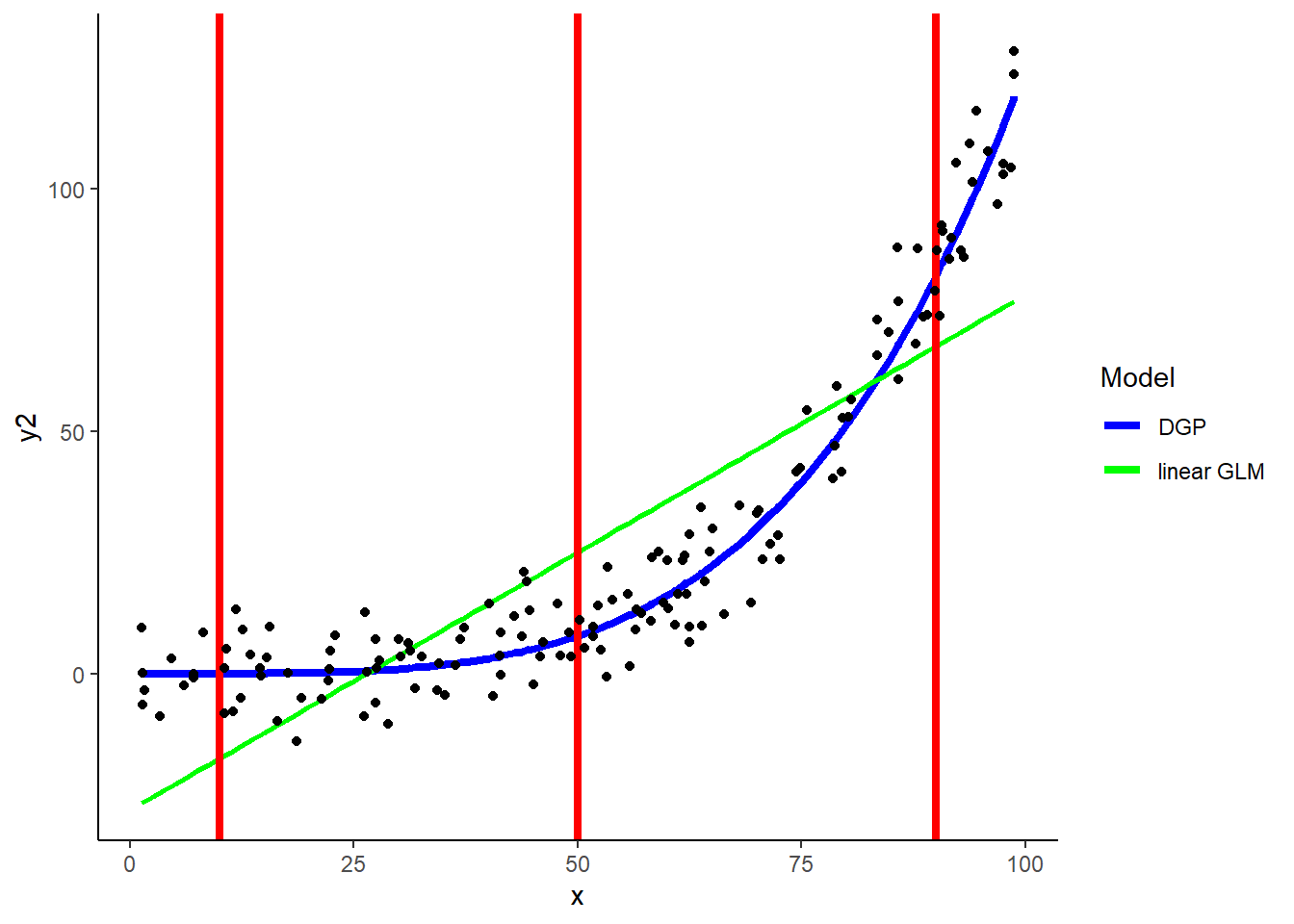
A simple example with simulated data from linear DGP of one predictor
Includes:
- DGP
- Simple linear model
- Red lines to represent three new observations (X = 10, 50, 90) to generate predictions via KNN
- What would 5-NN predictions look like for each of these three new values of X?

KNN can easily accommodate non-linear relationships between predictors and outcomes
In fact, it can flexibly handle ANY shape of relationship
ggplot(data = demo, aes(x = x, y = y3)) +
  geom_line(aes(x = x, y = y3_dgp, color = "blue"), size = 1.5) +
  geom_smooth(aes(color = "green"), method='lm',formula=y ~ x,  se = FALSE) +
  geom_vline(xintercept = 10, color = "red", size = 1.5)+
  geom_vline(xintercept = 50, color = "red", size = 1.5)+
  geom_vline(xintercept = 90, color = "red", size = 1.5) +
  geom_point(aes(y = y3), color = "black") +
  scale_color_identity(name = "Model",
                     breaks = c("blue", "green"),
                     labels = c("DGP", "linear GLM"),
                     guide = "legend")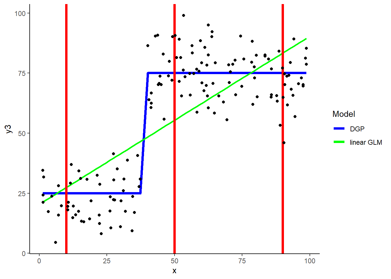
2.4.1 The hyperparameter k
KNN is our first example of a statistical model that includes a model hyperparameter, in this case ‘k’
Model hyperparameters differ from parameters in that they cannot be estimated while fitting the model to the training dataset
They must be set in advance
k = 5 is the default for knn in caret
Using the quadratic demo, 5-NN yields these predictions
##   k
## 1 5demo$y2_hat_k5 <- predict(knn_y2, demo)
ggplot(data = demo, aes(x = x, y = y2)) +
geom_line(aes(x = x, y = y2_dgp, color = "blue"), size = 1.5) +
geom_line(aes(x = x, y = y2_hat_k5, color = "red"), size = 1.5) +
geom_point(aes(y = y2), color = "black") +
scale_color_identity(name = "Model",
breaks = c("blue", "red"),
labels = c("DGP", "k = 5"),
guide = "legend")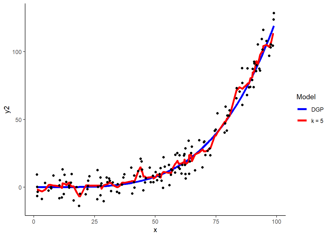
How will the size of k influence model performance (e.g., bias, variance)?
- Smaller values of k will tend to increase variance but decrease bias. Larger values of k will tend to decrease variance but increase bias. Need to find the sweet spot
How will k = 1 perform in training and test sets?
- k = 1 will perfectly fit the training set. Therefore it is very dependent on the training set (high variance). Clearly it will likely not do as well in test (it will be overfit to training). K needs to be larger if there is more noise (to average over more cases). K needs to be smaller if the relationships are complex. (More on choosing k by cross validation in later unit.)
k = 1
## # A tibble: 1 x 1
##       k
##   <dbl>
## 1     1
knn_y2_k1 <- train(y2 ~ x, data = demo,
method = "knn", trControl = trn_ctrl, tuneGrid = tune_grid)
demo$y2_hat_k1 <- predict(knn_y2_k1, demo)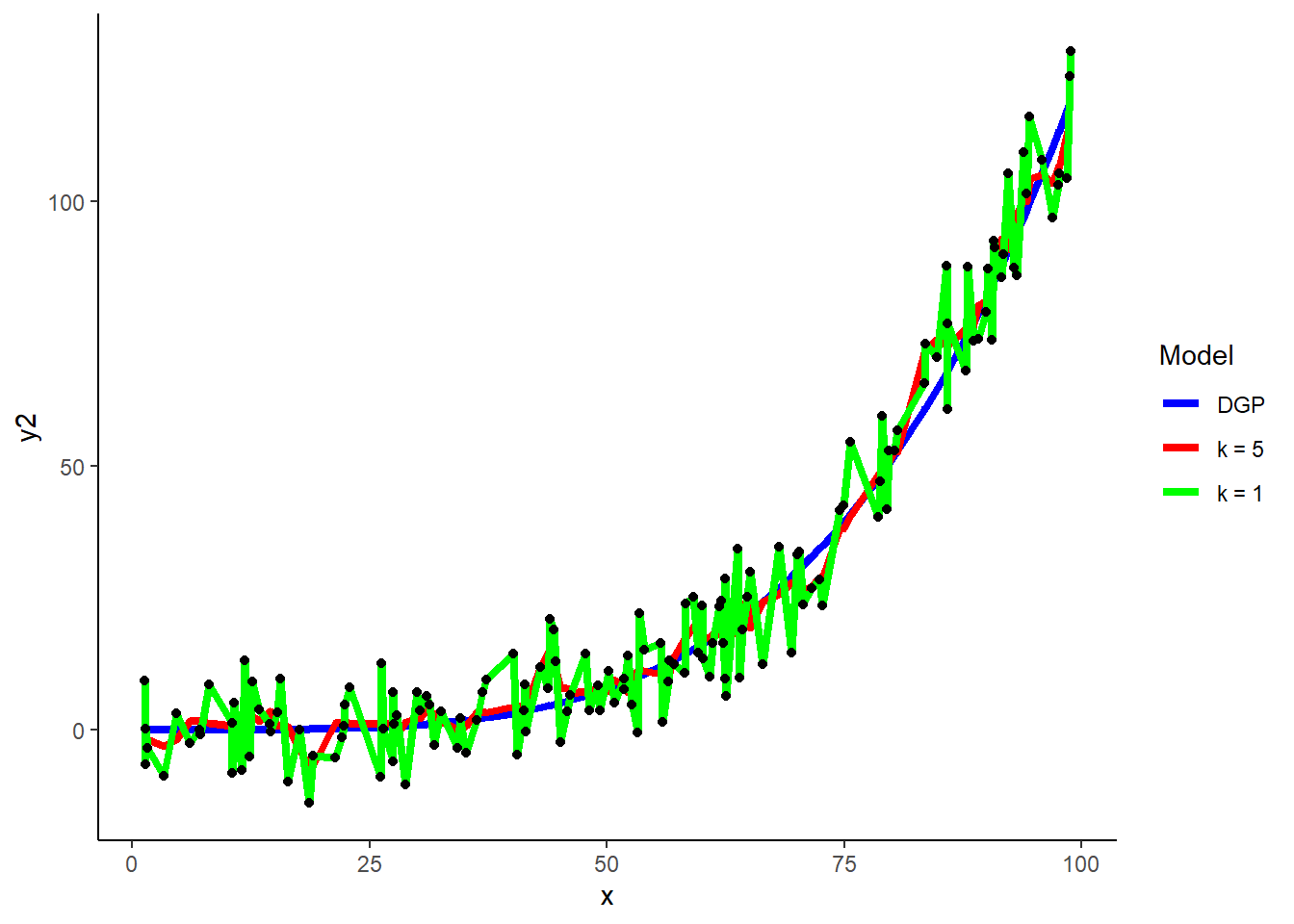
k = 75
tune_grid <- crossing(k = 75)

knn_y2_k75 <- train(y2 ~ x, data = demo,
            method = "knn", trControl = trn_ctrl, tuneGrid = tune_grid)

demo$y2_hat_k75 <- predict(knn_y2_k75, demo)
2.4.2 Defining “Nearest”
To make a prediction for some new observation, we need to identify the observations from the training set that are nearest to it
Need a distance measure to define “nearest”
There are a number of different distance measures available (e.g., Euclidean, Cosine, Chi square, Minkowsky)
Euclidean is most commonly used in KNN (and what is used by knn in caret)
IMPORTANT: We care only about:
- Distance between a test observation and all the training observations
- Need to find the k observation in training that are nearest to the test observation
- Distance is defined based on these observations features (predictors), not their outcomes
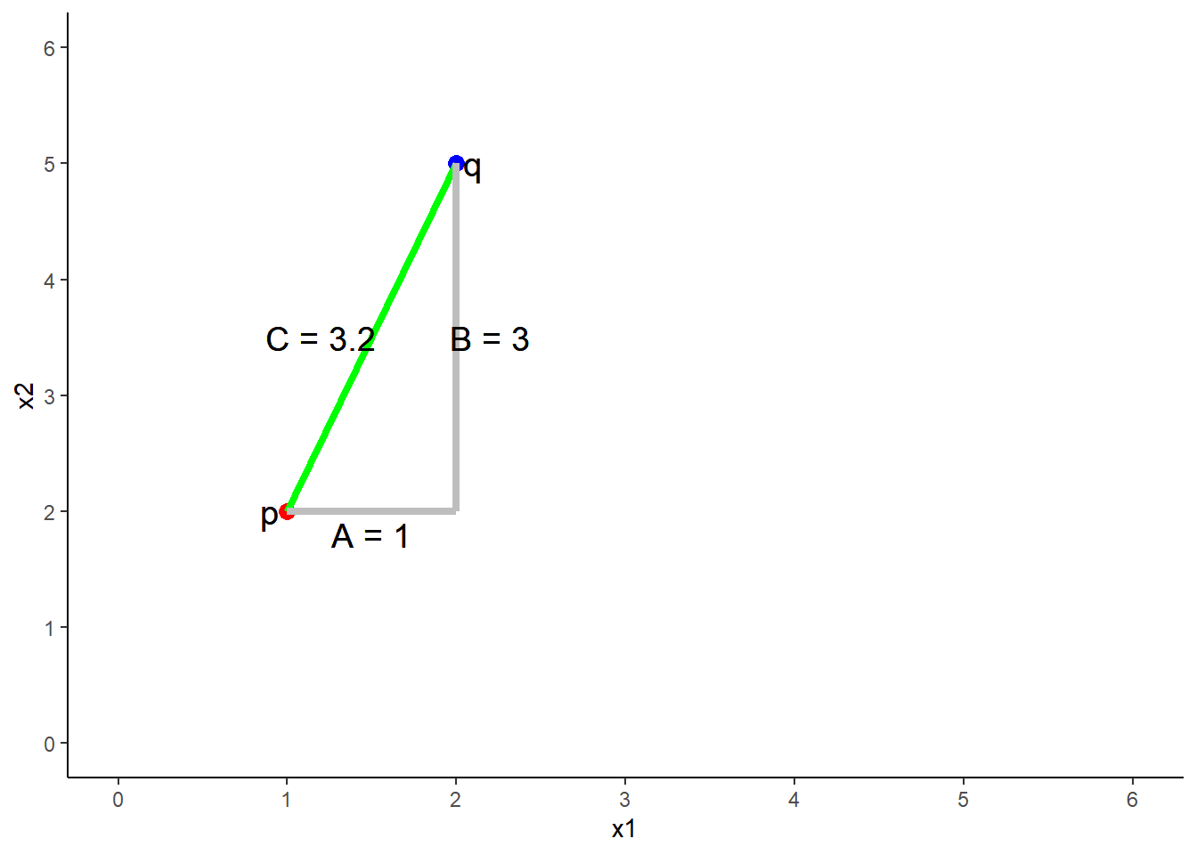
Euclidean distance between any two points is an n-dimensional extension of the Pythagorean formula (which applies explicitly with 2 predictors/2 dimensional space).
\(C^2 = A^2 + B^2\)
\(C = \sqrt{A^2 + B^2}\)
…where C is the distance between two points
The distance between 2 points (p and q) in two dimensions (2 predictors, x1 = A, x2 = B)
\(C = \sqrt{A^2 + B^2}\)
\(Distance = \sqrt{(q1 - p1)^2 + (q2 - p2)^2}\)
\(Distance = \sqrt{(2 - 1)^2 + (5 - 2)^2}\)
\(Distance = 3.2\)
One dimensional (one predictor) is simply the subtraction of scores on that predictor (x1) between p and q
\(Distance = \sqrt{(q1 - p1)^2}\)
\(Distance = \sqrt{(2 - 1)^2}\)
\(Distance = 1\)

N-dimensional generalization for n predictors:
\(Distance = \sqrt{(q1 - p1)^2 + (q2 - p2)^2 + ... + (qn - pn)^2}\)
2.4.3 Normalization of X
Distance is dependent on scales of all the predictors
We need to put all on the same scale
For quantitative variables: typically range correct to put on [0, 1] scale. For any x:
\[ x = \frac{x_i - min(x)}{max(x) - min(x)}\]
- KNN accommodates categorical variables as dummy variables
- Dummy variables are already on this scale so no need normalize or change scale in other way
2.4.4 KNN with Ames Housing Prices
Lets first start with fresh load of ames and splits
ames <- read_csv(file.path(data_path, "ames.csv")) %>%
  clean_names(case = "snake") %>%
  select(-id) %>%
  select(sale_price,
         gr_liv_area,
         lot_area,
         year_built,
         overall_qual,
         garage_cars,
         ms_zoning,
         lot_config,
         bldg_type) %>%
  mutate(ms_zoning = as.factor(ms_zoning),
         lot_config = as.factor(lot_config),
         bldg_type = as.factor(bldg_type))

contrasts(ames$ms_zoning) <- contr.treatment(length(levels(ames$ms_zoning)))
contrasts(ames$lot_config) <- contr.treatment(length(levels(ames$lot_config)))
contrasts(ames$bldg_type) <- contr.treatment(length(levels(ames$bldg_type)))

#Option to add explicit dummy codes instead of setting contrasts
# dmy_codes <- dummyVars(~ ms_zoning + lot_config + bldg_type, fullRank = TRUE, sep = "_", data = ames)
# ames <- ames %>%
#   bind_cols(as_tibble(predict(dmy_codes, ames))) %>%
#   select_if(is.numeric)

set.seed(19690127)
ames_splits <- initial_split(ames, prop = .8, strata = "sale_price")
train_knn <- training(ames_splits)
test_knn <- testing(ames_splits)
Normalize all quantitative variables to [0,1]
Dummy variables dont need to be normalized b/c they are already in the range of [0, 1]
All statistics for transformations need to be based on training dataset
In this case, that is the min and max of each variable that will be normalized
This same normalization formula will then be applied to test using min and max based on train
## Created from 1170 samples and 9 variables
##
## Pre-processing:
##   - ignored (3)
##   - re-scaling to [0, 1] (6)
train_knn_norm <- predict(normalize, train_knn) %>%
mutate(sale_price = train_knn$sale_price) %>%
glimpse()## Observations: 1,170
## Variables: 9
## $ sale_price <dbl> 208500, 223500, 143000, 307000, 129900, 118000, 129500, 144000, 157…
## $ gr_liv_area <dbl> 0.3169047, 0.3344081, 0.2367573, 0.3132197, 0.3316444, 0.1711193, 0…
## $ lot_area <dbl> 0.04376836, 0.06090842, 0.07844638, 0.05377081, 0.02950539, 0.03746…
## $ year_built <dbl> 0.9492754, 0.9347826, 0.8768116, 0.9565217, 0.4275362, 0.4855072, 0…
## $ overall_qual <dbl> 0.6666667, 0.6666667, 0.4444444, 0.7777778, 0.6666667, 0.4444444, 0…
## $ garage_cars <dbl> 0.50, 0.50, 0.50, 0.50, 0.50, 0.25, 0.25, 0.25, 0.25, 0.50, 0.50, 0…
## $ ms_zoning <fct> RL, RL, RL, RL, RM, RL, RL, RL, RL, RM, RL, RL, RL, RL, RM, RL, RM,…
## $ lot_config <fct> Inside, Inside, Inside, Inside, Inside, Corner, Inside, Inside, Cor…
## $ bldg_type <fct> 1Fam, 1Fam, 1Fam, 1Fam, 1Fam, 2fmCon, 1Fam, 1Fam, 1Fam, 1Fam, Duple…test_knn_norm <- predict(normalize, test_knn) %>%
mutate(sale_price = test_knn$sale_price) %>%
glimpse()## Observations: 290
## Variables: 9
## $ sale_price <dbl> 181500, 140000, 250000, 200000, 345000, 279500, 149000, 277500, 239…
## $ gr_liv_area <dbl> 0.21372639, 0.31851681, 0.42929526, 0.40442193, 0.45831414, 0.26715…
## $ lot_area <dbl> 0.05080803, 0.05050196, 0.07933399, 0.05559500, 0.06503428, 0.05724…
## $ year_built <dbl> 0.7536232, 0.3115942, 0.9275362, 0.7318841, 0.9637681, 0.9710145, 0…
## $ overall_qual <dbl> 0.5555556, 0.6666667, 0.7777778, 0.6666667, 0.8888889, 0.6666667, 0…
## $ garage_cars <dbl> 0.50, 0.75, 0.75, 0.50, 0.75, 0.75, 0.50, 0.50, 0.50, 0.50, 0.50, 0…
## $ ms_zoning <fct> RL, RL, RL, RL, RL, RL, RL, RL, RL, FV, RL, RL, RL, RL, RL, RL, RM,…
## $ lot_config <fct> FR2, Corner, FR2, Corner, Inside, Inside, CulDSac, Inside, CulDSac,…
## $ bldg_type <fct> 1Fam, 1Fam, 1Fam, 1Fam, 1Fam, 1Fam, 1Fam, TwnhsE, 1Fam, Twnhs, 1Fam…Why do we need to use only training to calculate the min and max for normalization?
- The model never ‘sees’ the test data because those are novel data so nothing about the model (even data pre-processing can depend on test data). Critical to enforce this or you will get bleed through into the test set and your estimate of model performance in new data may be overly optimistic!
But earlier, we calculated dummy codes using the full data before splitting into train/test. Why is that not a problem?
- The dummy codes in train dont change based on the data in test. Therefore, the model calculated in train isnt biased to better fit the test because of this. We do this so that train and test both have all the same dummy variables based on all possible levels of the categorical variable. However, if a dummy level doesnt exist in one of the sets, its dummy associated variable will be constant and not useful in that dataset.
Train a model using only quantitative variables
- k = 5
- NOTE: Still using same trn_ctrl as earlier with glm
knn5_quant <- train(sale_price ~ gr_liv_area + lot_area + year_built + overall_qual + garage_cars, data = train_knn_norm,
            method = "knn", trControl = trn_ctrl)

knn5_quant$bestTune
## k
## 1 5rmse_train_knn5_quant <- RMSE(predict(knn5_quant, train_knn_norm), train_knn_norm$sale_price)
rmse_test_knn5_quant <- RMSE(predict(knn5_quant, test_knn_norm), test_knn_norm$sale_price)
rmse <- bind_rows(rmse, tibble(model = "knn w/quant , k = 5", rmse_train = rmse_train_knn5_quant, rmse_test = rmse_test_knn5_quant))
kable(rmse)| model | rmse_train | rmse_test |
|---|---|---|
| simple regression | 56228.15 | 55871.92 |
| multiple regression | 38663.97 | 40789.77 |
| multiple regression w/categorical | 37700.56 | 39958.26 |
| multiple regression w/focal interaction | 36060.21 | 40673.83 |
| multiple regression w/all quant interactions | 32212.91 | 31747.06 |
| multiple regression w/all interactions | 29716.56 | 39941.31 |
| best? multiple regression | 31417.38 | 31045.39 |
| knn w/quant , k = 5 | 28783.70 | 38973.74 |
It is often useful (for any model) to compare predicted to observed outcome
Do this in training or you run the risk of changing your model to fit test (or otherwise, use yet another test. More on this later)
sp <- tibble(predicted = predict(knn5_quant, train_knn_norm),
             observed = train_knn_norm$sale_price)
ggplot(data = sp, aes(x = predicted, y = observed)) +
  geom_point()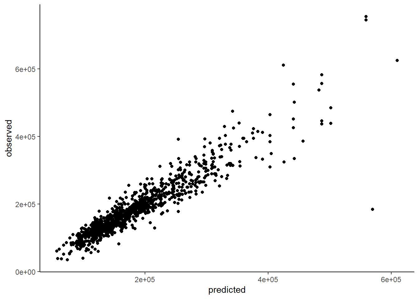
Try k = 20 & 50
- NOTE use of tune_grid in \(train()\)
#k = 20
tune_grid <- expand.grid(k = 20)
knn20_quant <- train(sale_price ~ gr_liv_area + lot_area + year_built + overall_qual + garage_cars, data = train_knn_norm,
            method = "knn", trControl = trn_ctrl , tuneGrid = tune_grid)

rmse_train_knn20_quant <- RMSE(predict(knn20_quant, train_knn_norm), train_knn_norm$sale_price)
rmse_test_knn20_quant <- RMSE(predict(knn20_quant, test_knn_norm), test_knn_norm$sale_price)
rmse <- bind_rows(rmse, tibble(model = "knn w/quant , k = 20", rmse_train = rmse_train_knn20_quant, rmse_test = rmse_test_knn20_quant))

#k = 50
tune_grid <- expand.grid(k = 50)
knn50_quant <- train(sale_price ~ gr_liv_area + lot_area + year_built + overall_qual + garage_cars, data = train_knn_norm,
            method = "knn", trControl = trn_ctrl , tuneGrid = tune_grid)

rmse_train_knn50_quant <- RMSE(predict(knn50_quant, train_knn_norm), train_knn_norm$sale_price)
rmse_test_knn50_quant <- RMSE(predict(knn50_quant, test_knn_norm), test_knn_norm$sale_price)
rmse <- bind_rows(rmse, tibble(model = "knn w/quant , k = 50", rmse_train = rmse_train_knn50_quant, rmse_test = rmse_test_knn50_quant))
What is going on with train and test error across the three levels of k we considered?
- As k increases, the models fit worse in training but better in test. This is because the lower k values are overfit to training. There is some bias introduced as k increases but its overcome by the reduction in variance.
| model | rmse_train | rmse_test |
|---|---|---|
| simple regression | 56228.15 | 55871.92 |
| multiple regression | 38663.97 | 40789.77 |
| multiple regression w/categorical | 37700.56 | 39958.26 |
| multiple regression w/focal interaction | 36060.21 | 40673.83 |
| multiple regression w/all quant interactions | 32212.91 | 31747.06 |
| multiple regression w/all interactions | 29716.56 | 39941.31 |
| best? multiple regression | 31417.38 | 31045.39 |
| knn w/quant , k = 5 | 28783.70 | 38973.74 |
| knn w/quant , k = 20 | 34056.31 | 35501.02 |
| knn w/quant , k = 50 | 38649.48 | 34954.15 |
We can add the categorical variables to the model
We can use ‘.’ because now using all predictors in train_knn_norm
#k = 5
knn5_all <- train(sale_price ~ ., data = train_knn_norm,
            method = "knn", trControl = trn_ctrl)

rmse_train_knn5_all <- RMSE(predict(knn5_all, train_knn_norm), train_knn_norm$sale_price)
rmse_test_knn5_all <- RMSE(predict(knn5_all, test_knn_norm), test_knn_norm$sale_price)
rmse <- bind_rows(rmse, tibble(model = "knn w/all , k = 5", rmse_train = rmse_train_knn5_all, rmse_test = rmse_test_knn5_all))

#k = 20
tune_grid <- expand.grid(k = 20)
knn20_all <- train(sale_price ~ ., data = train_knn_norm,
            method = "knn", trControl = trn_ctrl , tuneGrid = tune_grid)

rmse_train_knn20_all <- RMSE(predict(knn20_all, train_knn_norm), train_knn_norm$sale_price)
rmse_test_knn20_all <- RMSE(predict(knn20_all, test_knn_norm), test_knn_norm$sale_price)
rmse <- bind_rows(rmse, tibble(model = "knn w/all , k = 20", rmse_train = rmse_train_knn20_all, rmse_test = rmse_test_knn20_all))

#k = 50
tune_grid <- expand.grid(k = 50)
knn50_all <- train(sale_price ~ ., data = train_knn_norm,
            method = "knn", trControl = trn_ctrl , tuneGrid = tune_grid)

rmse_train_knn50_all <- RMSE(predict(knn50_all, train_knn_norm), train_knn_norm$sale_price)
rmse_test_knn50_all <- RMSE(predict(knn50_all, test_knn_norm), test_knn_norm$sale_price)
rmse <- bind_rows(rmse, tibble(model = "knn w/all , k = 50", rmse_train = rmse_train_knn50_all, rmse_test = rmse_test_knn50_all))

kable(rmse)| model | rmse_train | rmse_test |
|---|---|---|
| simple regression | 56228.15 | 55871.92 |
| multiple regression | 38663.97 | 40789.77 |
| multiple regression w/categorical | 37700.56 | 39958.26 |
| multiple regression w/focal interaction | 36060.21 | 40673.83 |
| multiple regression w/all quant interactions | 32212.91 | 31747.06 |
| multiple regression w/all interactions | 29716.56 | 39941.31 |
| best? multiple regression | 31417.38 | 31045.39 |
| knn w/quant , k = 5 | 28783.70 | 38973.74 |
| knn w/quant , k = 20 | 34056.31 | 35501.02 |
| knn w/quant , k = 50 | 38649.48 | 34954.15 |
| knn w/all , k = 5 | 30567.56 | 38193.47 |
| knn w/all , k = 20 | 41078.22 | 34963.19 |
| knn w/all , k = 50 | 47942.01 | 37887.09 |
2.5 Programming Tips
caret package:
- \(train()\)
- \(RMSE()\)
- \(predict()\)
- \(dummyVars()\)
- \(preProcess(., method = range)\)
rsample package:
- \(initial_split()\)
- \(training()\)
- \(testing()\)
Tidyverse:
- \(select()\)
- \(rename()\)
- \(filter()\)
- \(arrange()\)
- \(mutate()\)
- \(group_by()\)
- \(summarise()\)