3 Introduction to Classification Models
3.1 Unit overview
We will cover the following topics in this unit:
- Bayes classifier
- Logistic regression
- K nearest neighbors
- Linear discriminant analysis
- Quadratic discriminant analysis
- Classification model performance metrics
- Confusion matrices
- Accuracy
- Sensitivity, specificity, PPV and NPV
- f1 and balance accuracy
- Kappa
3.2 Bayes classifier
The figure below displays simulated data for a classification problem for K = 2 classes as a function of \(X_1\) and \(X_2\)
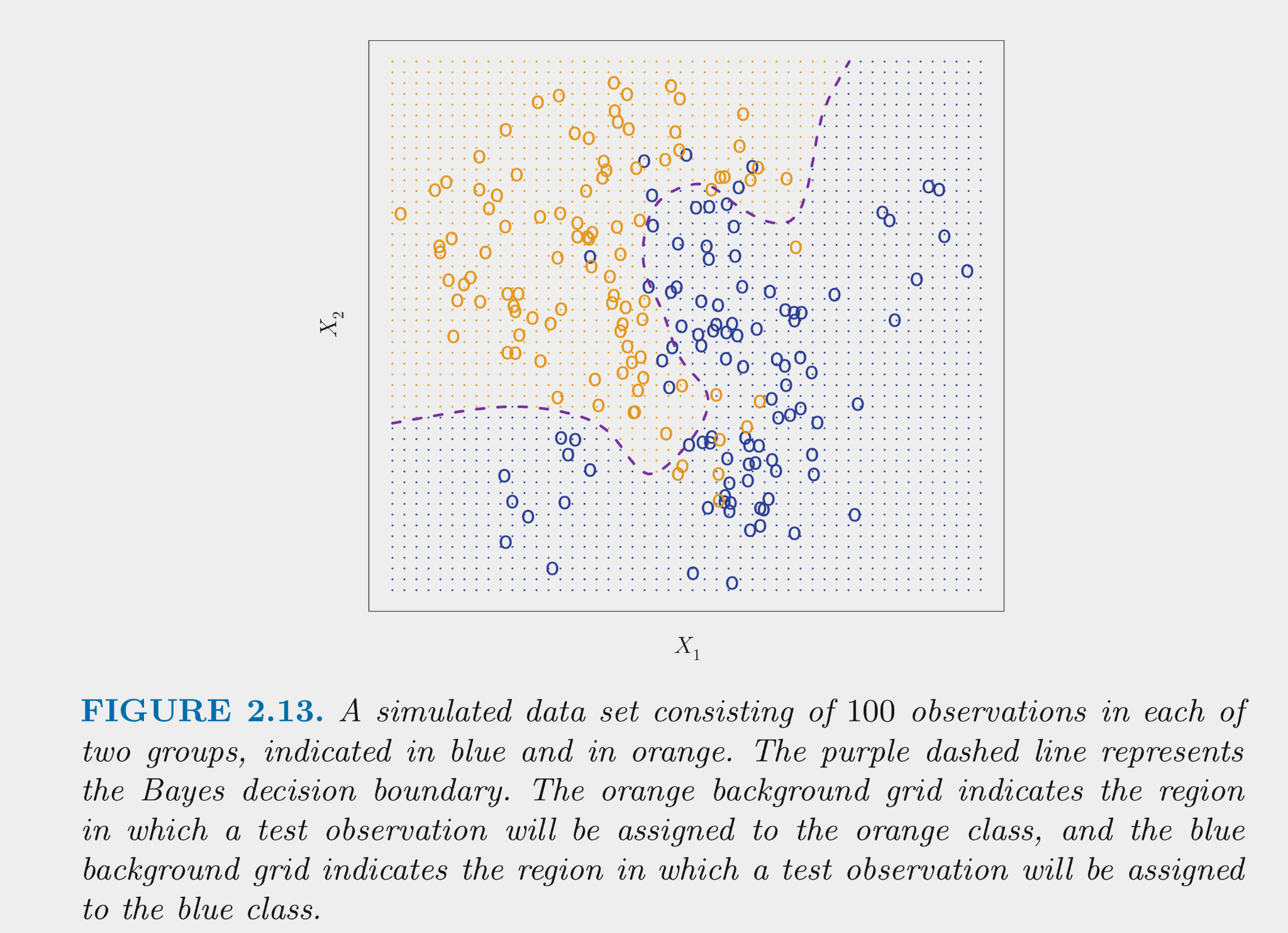
The Bayes classifier assigns each observation its most likely class given its conditional probabilities for the values for \(X_1\) and \(X_2\)
- \(Pr(Y = k | X = x_0) for\:k = 1:K\)
- For K = 2, this means assigning to the class with Pr > .50
- This decision boundary for the two class problem is displayed in the figure
The Bayes classifier provides the minimum error rate for test data
- Error rate for any \(x_0\) will be \(1 - max (Pr( Y = k | X = x_0))\)
- Overall error rate will be the average of this across all possible X
- This is the irreducible error for classification problems
- This is a theoretical model b/c (except for simulated data), we dont know the conditional probabilities based on X
- Many classification models try to estimate these conditionals
Lets talk now about some of these classification models
3.3 Logistic regression
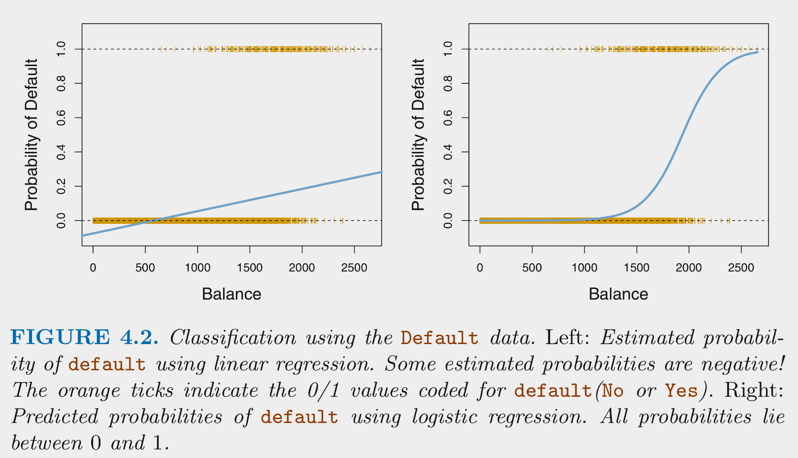
Logistic regression estimates the conditional probability for each class given X
Why not use a general linear model?
- The general linear model would make probability predictions that are not bounded by [0, 1]. Also couldnt code multi-class outcomes with a single variable (e.g., Y = 1, 2, or 3) unless the classes were ordered. The logistic model is superior.
Logistic regression provides predicted conditional probabilities for one class (positive class) for any specific set of values on predictors (X)
\[Pr(positive\:class | X) = \frac{e^{\beta_0 + \beta_1*X_1 + \beta_2*X_2 + ... + \beta_p * X_p}}{1 + e^{\beta_0 + \beta_1*X_1 + \beta_2*X_2 + ... + \beta_p * X_p}}\]
These conditional probabilities are bounded by [0, 1]
To maximize accuracy (as per Bayes classifier), predict the positive case if Pr(positive case | X) > .5 for any specific X, otherwise predict the negative case.
In some instances, it may make more sense to describe the odds of the positive case occurring (e.g., horse racing) rather than probability
Odds are defined with respect to probabilities as follows:
\[odds = \frac{Pr(positive\:class|X)} {1 - Pr(positive\:class|X)}\]
Examples of odds calculations:
\[odds = \frac{Pr(positive\:class|X)} {1 - Pr(positive\:class|X)}\]
If the UW Badgers have a .5 probability of winning some upcoming game based on X, what are their odds of winning ?
- Their odds of winning are 1 (to 1)
If the UW Badgers have a .75 probability of winning some upcoming game based on X, what are their odds of winning ?
- Their odds of winning are 3 (:1; ‘3 to 1’)
If the UW Badgers have a .25 probability of winning some upcoming game based on X, what are their odds of winning ?
- Their odds of winning are .33 (1:3)
The logistic function can be modified to provide odds directly:
Logistic function: \[Pr(positive\:class | X) = \frac{e^{\beta_0 + \beta_1*X_1 + \beta_2*X_2 + ... + \beta_p * X_p}}{1 + e^{\beta_0 + \beta_1*X_1 + \beta_2*X_2 + ... + \beta_p * X_p}}\]
Definition of odds:
\[odds = \frac{Pr(positive\:class|X)} {1 - Pr(positive\:class|X)}\]
Substitute logistic function for \(Pr(positive\:class|X)\) on top and bottom and simplify to get:
\[odds(positive\:class|X) = e^{\beta_0 + \beta_1*X_1 + \beta_2*X_2 + ... + \beta_p * X_p}\]
Odds are bounded by [0, \(\infty\)]
The logistic function can be modified further such that the outcome (log-odds/logit) is a linear function of X
Take the natural log (base e) of both sides of the odds equation:
\[log(odds(positive\:class|X)) = \beta_0 + \beta_1*X_1 + \beta_2*X_2 + ... + \beta_p * X_p\]
Log-odds are unbounded \([-\infty, \infty]\)
Use of logit transformation provides the connection between the general linear model and generalized linear models (in this case with link = logit, family = binomial)
Odds and probability are descriptive but they are not linear functions of X
- Therefore, parameter estimates from these models arent very useful to describe effect of any x in X
- This is because unit change in Y per unit change in x is not the same for all values of x
Log-odds are linear function of X
- Therefore, you can say that log-odds of positive class increases by \(\beta_1\) for every one unit increase in \(x_1\)
- However, log-odds are NOT very descriptive/intuitive so not that useful for understanding
So how can we describe the effects of any x in X?
- We can use the ‘odds ratio’
Odds are defined at a specific set of values across predictors in X. For example, with one predictor:
\[odds = \frac{Pr(positive\:class|x_1)} {1 - Pr(positive\:class|x_1)}\]
The odds ratio describes the change in odds for a change of c units in any x in X
\[Odds\:ratio = \frac{odds(x+c)}{odds(x)}\]
\[Odds\:ratio = \frac{e^{\beta_0 + \beta_1*(x_1 + c)}}{e^{\beta_0 + \beta_1*x_1}}\] \[Odds\:ratio = e^{c*\beta_1}\]
Lets put it all together in the Auto dataset from the package from ISL
library(caret)
library(tidyverse)
library(rsample)
library(ISLR)

auto <- as_tibble(Auto) %>%
  mutate(high_mpg = if_else(mpg > median(mpg),1,0), #make a high/low mpg variable to demo classification
         high_mpg = factor(high_mpg, levels = c(0,1), labels = c("low", "high"))) %>%
  select(-mpg) %>%
  glimpse()
## Observations: 392
## Variables: 9
## $ cylinders <dbl> 8, 8, 8, 8, 8, 8, 8, 8, 8, 8, 8, 8, 8, 8, 4, 6, 6, 6, 4, 4, 4, 4, 4…
## $ displacement <dbl> 307, 350, 318, 304, 302, 429, 454, 440, 455, 390, 383, 340, 400, 45…
## $ horsepower <dbl> 130, 165, 150, 150, 140, 198, 220, 215, 225, 190, 170, 160, 150, 22…
## $ weight <dbl> 3504, 3693, 3436, 3433, 3449, 4341, 4354, 4312, 4425, 3850, 3563, 3…
## $ acceleration <dbl> 12.0, 11.5, 11.0, 12.0, 10.5, 10.0, 9.0, 8.5, 10.0, 8.5, 10.0, 8.0,…
## $ year <dbl> 70, 70, 70, 70, 70, 70, 70, 70, 70, 70, 70, 70, 70, 70, 70, 70, 70,…
## $ origin <dbl> 1, 1, 1, 1, 1, 1, 1, 1, 1, 1, 1, 1, 1, 1, 3, 1, 1, 1, 3, 2, 2, 2, 2…
## $ name <fct> chevrolet chevelle malibu, buick skylark 320, plymouth satellite, a…
## $ high_mpg <fct> low, low, low, low, low, low, low, low, low, low, low, low, low, lo…Make training and test data with 75% in train, stratified on outcome
set.seed(20110522)
auto_splits <- initial_split(auto, prop = .75, strata = "high_mpg")
trn <- training(auto_splits)
test <- testing(auto_splits)
dim(trn)## [1] 294 9## [1] 98 9Any concerns about using training-test split for cross validation?
- These samples are starting to get a little small. Trained model will have higher variance with only 75% (N = 294) observations and performance in test (with only N = 98 observations) may not be a very precise estimate of true test error.
Lets examine the effects of engine displacement and production year
trn_ctrl <- trainControl(method = "none")
lr1 <- train(high_mpg ~ displacement + year, data = trn,
method = "glm", family = "binomial", trControl = trn_ctrl)
summary(lr1)##
## Call:
## NULL
##
## Deviance Residuals:
## Min 1Q Median 3Q Max
## -2.6415 -0.1873 0.0671 0.3840 3.2158
##
## Coefficients:
## Estimate Std. Error z value Pr(>|z|)
## (Intercept) -16.055474 4.598396 -3.492 0.00048 ***
## displacement -0.036249 0.004529 -8.004 1.20e-15 ***
## year 0.291080 0.063756 4.566 4.98e-06 ***
## ---
## Signif. codes: 0 '***' 0.001 '**' 0.01 '*' 0.05 '.' 0.1 ' ' 1
##
## (Dispersion parameter for binomial family taken to be 1)
##
## Null deviance: 407.57 on 293 degrees of freedom
## Residual deviance: 148.80 on 291 degrees of freedom
## AIC: 154.8
##
## Number of Fisher Scoring iterations: 7\[Pr(high\:|displacement) = \frac{e^{-16.06 -.03*displacement + .29*year}}{1 + e^{-16.06 -.03*displacement + .29*year}}\]
Use \(predict()\) to get these probabilities (or predicted class) directly from the model for any data
- Predicted class based on 50% threshold
Lets examine the effect of \(displacement\) holding \(year\) constant at its mean
new_displacements <- tibble(displacement = seq(min(trn$displacement), max(trn$displacement),1), year = mean(trn$year))
new_displacements$pr_high <- predict(lr1, new_displacements, type = "prob")$high
new_displacements$pr_high[1:10]## [1] 0.9735238 0.9725732 0.9715896 0.9705717 0.9695185 0.9684288 0.9673015 0.9661354
## [9] 0.9649291 0.9636815new_displacements$pred_classes <- predict(lr1, new_displacements, type = "raw")
new_displacements$pred_classes[1:10]## [1] high high high high high high high high high high
## Levels: low highCan plot this relationship using the predicted probabilities
library(ggthemes)
theme_set(theme_classic())
ggplot(data=trn, aes(displacement, as.numeric(high_mpg) - 1)) +
geom_point(position = position_jitter(height = 0.03, width = 0)) +
geom_line(data = new_displacements, mapping = aes(x = displacement, y = pr_high)) +
xlab("Displacement") +
ylab("Pr(High MPG | Displacement)")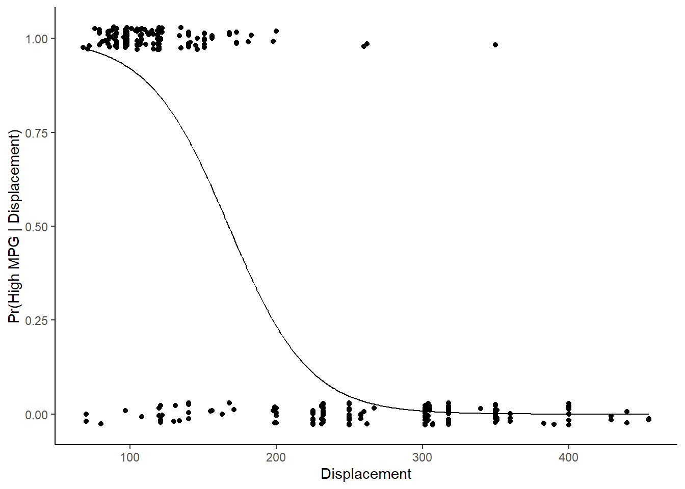
Can plot odds instead of probabilities using odds equation and coefficients from the model
\[odds(high\:mpg|X) = e^{-16.06 -.03*displacement + .29*year}\] NOTE: Use coefficient names rather than positions
## (Intercept) displacement year
## -16.05547449 -0.03624885 0.29108026new_displacements$odds1 <- exp(coef(lr1$finalModel)["(Intercept)"] +
coef(lr1$finalModel)["displacement"] * new_displacements$displacement +
coef(lr1$finalModel)["year"] * new_displacements$year)or by transforming probabilities into odds
\[odds = \frac{Pr(positive\:class|x_1)} {1 - Pr(positive\:class|x_1)}\]
NOTE: Harder to also plot raw data as scatter plot when plotting odds vs. probabilities. Maybe use second Y axis?
## # A tibble: 5 x 6
## displacement year pr_high pred_classes odds1 odds2
## <dbl> <dbl> <dbl> <fct> <dbl> <dbl>
## 1 68 76.0 0.974 high 36.8 36.8
## 2 69 76.0 0.973 high 35.5 35.5
## 3 70 76.0 0.972 high 34.2 34.2
## 4 71 76.0 0.971 high 33.0 33.0
## 5 72 76.0 0.970 high 31.8 31.8ggplot(data=trn, aes(displacement, as.numeric(high_mpg) - 1)) +
geom_line(data = new_displacements, mapping = aes(x = displacement, y = odds1)) +
xlab("Displacement") + ylab("Odds(High MPG | Displacement)")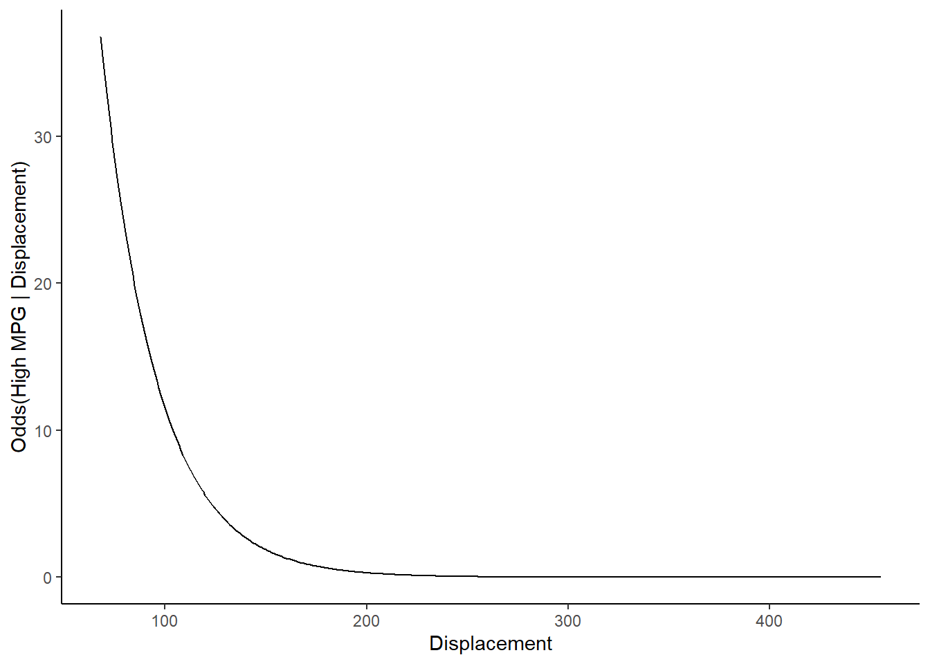
Odds ratio for displacement:
\[Odds\:ratio = e^{c*\beta_1}\]
## displacement
## 0.9644003For every one unit increase in displacement (holding year constant), the odds of a car being categorized as high mpg decrease by a factor of .97
You can do this for other values of c as well
\[Odds\:ratio = e^{c*\beta_1}\]
## displacement
## 0.6959424For every 10 unit increase in displacement (holding year constant), the odds of a car being categorized as high mpg decrease by a factor of .72
## displacement
## 0.02379667For every 1 standard deviation unit increase in displacement, the odds of a car being categorized as high mpg decrease by a factor of .03
We can also do this for year
Each of these odds ratios are controlling for all other predictors in the model
## year
## 1.337872For every 1 unit increase in production year (holding displacement constant), the odds of a car being categorized as high mpg increase by a factor of 1.34
How are categorical variables handled in logistic regression or generalized linear models more generally?
- Same as for linear models: dummy variables or other contrast codes
How are interactions handled in logistic regression or generalized linear models more generally?
- Same as for linear models: product terms
How are non-linear (with respect to logit) handled in logistic regression or generalized linear models more generally?
- Same as for linear models: polynomial terms or other transformations
FINALLY NOTE: Some tasks require fitting the final model using \(glm()\) because the associated R package/function only accepts lm/glm objects
Likelihood ratio test
- Note that outcome is coded 0,1
- Note type = 3 (not needed with simple regression but important when interactions are present)
glm1 <- glm(as.numeric(high_mpg) - 1 ~ displacement + year, family = "binomial", data = trn)
library(car)
Anova(glm1, type = 3)## Analysis of Deviance Table (Type III tests)
##
## Response: as.numeric(high_mpg) - 1
## LR Chisq Df Pr(>Chisq)
## displacement 204.012 1 < 2.2e-16 ***
## year 25.257 1 5.018e-07 ***
## ---
## Signif. codes: 0 '***' 0.001 '**' 0.01 '*' 0.05 '.' 0.1 ' ' 1Use of predict.glm for SE
- Note \(type\), and \(se\)
- Can plot preds directly with se
- NOTE: use of type = “response” for use with \(predict.glm()\)
## [1] "fit" "se.fit" "residual.scale"## 1 2 3 4 5
## 2.323689e-04 7.408371e-04 1.322369e-03 1.326179e-05 8.900913e-06We didnt use the test set for anything in these analyses so far. What is test useful for?
- 1. Test set will allow us to estimate how well our model predicts in new data (prediction focus). 2. Test would allow us to choose the best model to test our parameters within. ‘Best’ means the model that most closely matches the DGP, which is also the model that provides the most accurate predictions. There may be other factors to consider when defining ‘Best’ for inference.
How accurate is our two predictor model?
Lets start by writing an accuracy function
Lets use this function to calculate model accuracy in train and test
Model accuracy in training
## [1] 0.9115646Model accuracy in test
## [1] 0.9081633Are you surprised that the model doesnt much fit worse in test?
- No. There are three sources of error in test: variance/overfitting, bias, and irreducible error. Irreducible error and bias are present to the same degree in both test and training. Overfitting errors will manifest only in test but this model isnt overfit. Big N, small p. Finally, there is less overfitting with strong predictors. These are pretty strong predictors of high_mpg
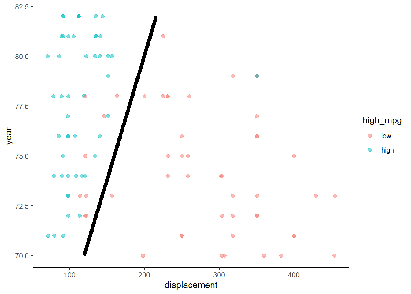
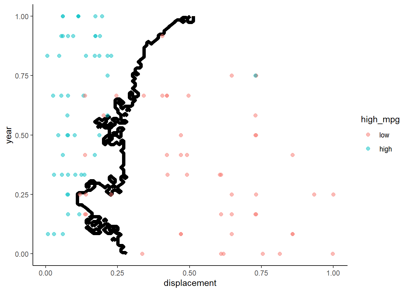
Lets take a look at the decision boundary in train and test for this model
What do we know about the decision boundary from a two predictor linear regression with a binary outcome?
- Logistic regression produces a linear decision boundary when you consider a scatter plot of the points by the two predictors. Points on one side of the line are assigned to one class and points on the other side of the line are assigned to the other class. This decision boundary would be a plane if there were three predictors. Harder to visualize in higher dimensional space.
First we need a function to plot the decision boundary because we will use it repeatedly to compare decision boundaries across statistical models
NOTE:
- Attempt to make function more flexible/generic RE variable names
- Use of argument (n_points) with default
plot_db <- function(model, data, x_names, y_name, n_points = 100) {
preds <- crossing(X1 = seq(min(data[[x_names[1]]]),
max(data[[x_names[1]]]),
length = n_points),
X2 = seq(min(data[[x_names[2]]]),
max(data[[x_names[2]]]),
length = n_points))
names(preds) <- x_names
preds[[y_name]] <- predict(model, preds)
preds[[y_name]] <- as.numeric(preds[[y_name]])-1
ggplot(data = data, aes(x = data[[x_names[1]]], y = data[[x_names[2]]], color = data[[y_name]])) +
geom_contour(data = preds, aes(x = preds[[x_names[1]]], y = preds[[x_names[2]]], z = preds[[y_name]]), color = "black", breaks = .5, size = 2) +
geom_point(size = 2, alpha = .5) +
labs(x = x_names[1], y = x_names[2], color = y_name)
}Here are the two decision boundary plots
- Training
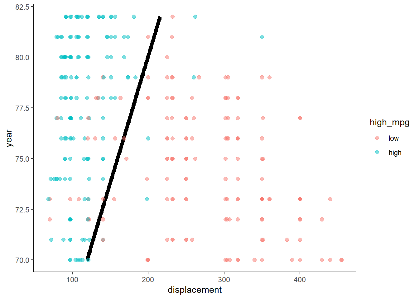
- Test
Lets consider the other predictors
Lets exclude name b/c there are MANY names and not coded very clearly
## Observations: 392
## Variables: 9
## $ cylinders    <dbl> 8, 8, 8, 8, 8, 8, 8, 8, 8, 8, 8, 8, 8, 8, 4, 6, 6, 6, 4, 4, 4, 4, 4…
## $ displacement <dbl> 307, 350, 318, 304, 302, 429, 454, 440, 455, 390, 383, 340, 400, 45…
## $ horsepower   <dbl> 130, 165, 150, 150, 140, 198, 220, 215, 225, 190, 170, 160, 150, 22…
## $ weight       <dbl> 3504, 3693, 3436, 3433, 3449, 4341, 4354, 4312, 4425, 3850, 3563, 3…
## $ acceleration <dbl> 12.0, 11.5, 11.0, 12.0, 10.5, 10.0, 9.0, 8.5, 10.0, 8.5, 10.0, 8.0,…
## $ year         <dbl> 70, 70, 70, 70, 70, 70, 70, 70, 70, 70, 70, 70, 70, 70, 70, 70, 70,…
## $ origin       <dbl> 1, 1, 1, 1, 1, 1, 1, 1, 1, 1, 1, 1, 1, 1, 3, 1, 1, 1, 3, 2, 2, 2, 2…
## $ name         <fct> chevrolet chevelle malibu, buick skylark 320, plymouth satellite, a…
## $ high_mpg <fct> low, low, low, low, low, low, low, low, low, low, low, low, low, lo…Do we need to do anything else to these predictors?
- Code origin with dummy coding.
Calculate explicit dummy variables so we can make correlation matrix
Put high_mpg first (my preference)
auto <- auto %>%
  select(-name) %>%
  mutate(origin = as.factor(origin))

dmy_codes <- dummyVars(~origin, sep = "_", fullRank = TRUE,
                       data = auto)
dmy_data <- as_tibble(predict(dmy_codes, auto))
auto <- auto %>%
  bind_cols (dmy_data) %>%
  select(-origin) %>%
  select(high_mpg, everything()) %>%
  glimpse()
## Observations: 392
## Variables: 9
## $ high_mpg <fct> low, low, low, low, low, low, low, low, low, low, low, low, low, lo…
## $ cylinders <dbl> 8, 8, 8, 8, 8, 8, 8, 8, 8, 8, 8, 8, 8, 8, 4, 6, 6, 6, 4, 4, 4, 4, 4…
## $ displacement <dbl> 307, 350, 318, 304, 302, 429, 454, 440, 455, 390, 383, 340, 400, 45…
## $ horsepower <dbl> 130, 165, 150, 150, 140, 198, 220, 215, 225, 190, 170, 160, 150, 22…
## $ weight <dbl> 3504, 3693, 3436, 3433, 3449, 4341, 4354, 4312, 4425, 3850, 3563, 3…
## $ acceleration <dbl> 12.0, 11.5, 11.0, 12.0, 10.5, 10.0, 9.0, 8.5, 10.0, 8.5, 10.0, 8.0,…
## $ year <dbl> 70, 70, 70, 70, 70, 70, 70, 70, 70, 70, 70, 70, 70, 70, 70, 70, 70,…
## $ origin_2 <dbl> 0, 0, 0, 0, 0, 0, 0, 0, 0, 0, 0, 0, 0, 0, 0, 0, 0, 0, 0, 1, 1, 1, 1…
## $ origin_3 <dbl> 0, 0, 0, 0, 0, 0, 0, 0, 0, 0, 0, 0, 0, 0, 1, 0, 0, 0, 1, 0, 0, 0, 0…Resplit using same seed as earlier
set.seed(20110522)
auto_splits <- initial_split(auto, prop = .75, strata = "high_mpg")
trn <- training(auto_splits)
test <- testing(auto_splits)
Look at correlations among predictors in training set (dont use test or full dataset!)
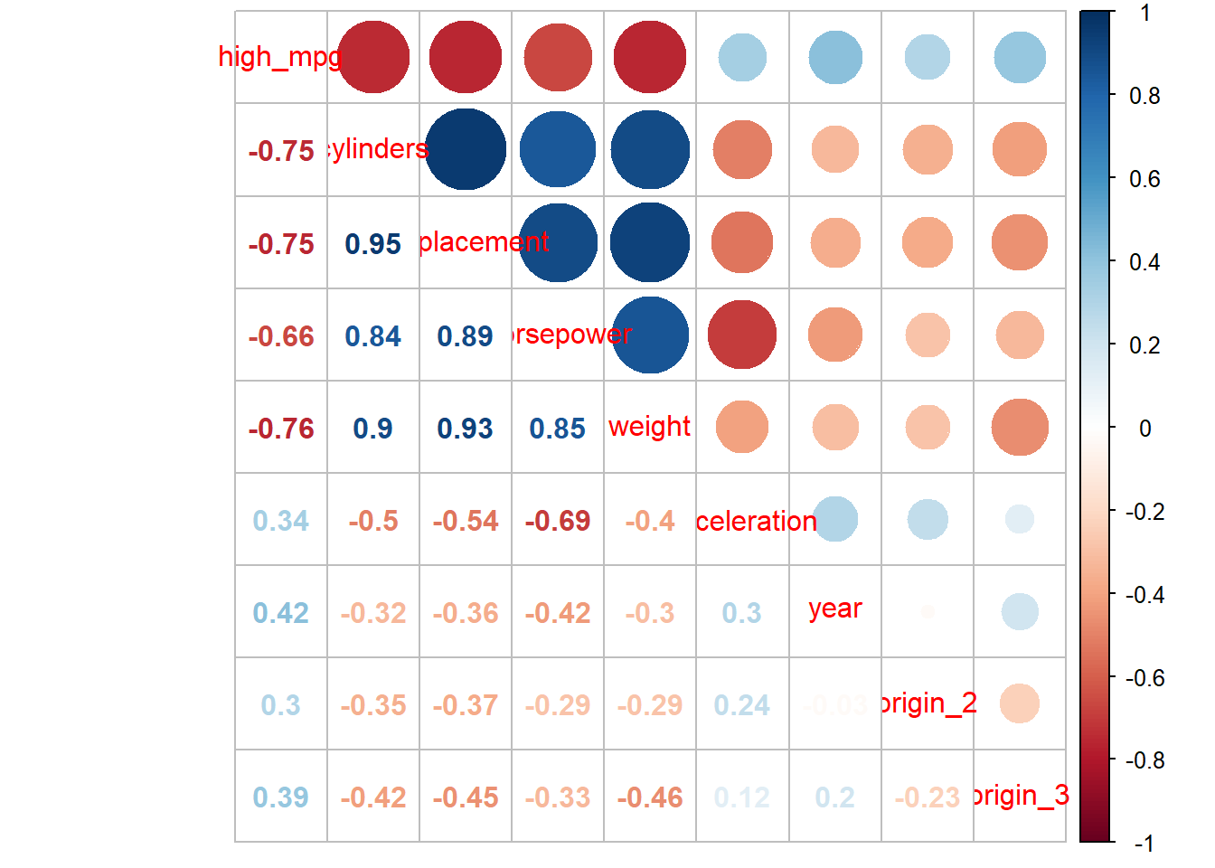
Do you think we can eek out more accuracy?
- We have a pretty good model and the remaining variables are pretty correlated (redundant) with our current predictors
lr_all <- train(high_mpg ~ ., data = trn,
             method = "glm", family = "binomial", trControl = trn_ctrl)
Model accuracy in training
## [1] 0.914966Model accuracy in test
## [1] 0.8979592This model fits descriptively worse than the 2 predictor model. Correlated predictors increase variance in general and generalized models.
What do highly correlated predictors do in the general linear model?
- High multi-collinearity inflates standard errors for parameter estimates. In other words, leads to high variance/overfit models that dont predict as well in new data!
3.4 K nearest neighbors
Lets switch gears to a non-parametric method we already know. KNN can be used as a classifier as well as for regression problems
KNN tries to determine conditional class possibilities for any X by looking at observed classes for similar values of X in the training set
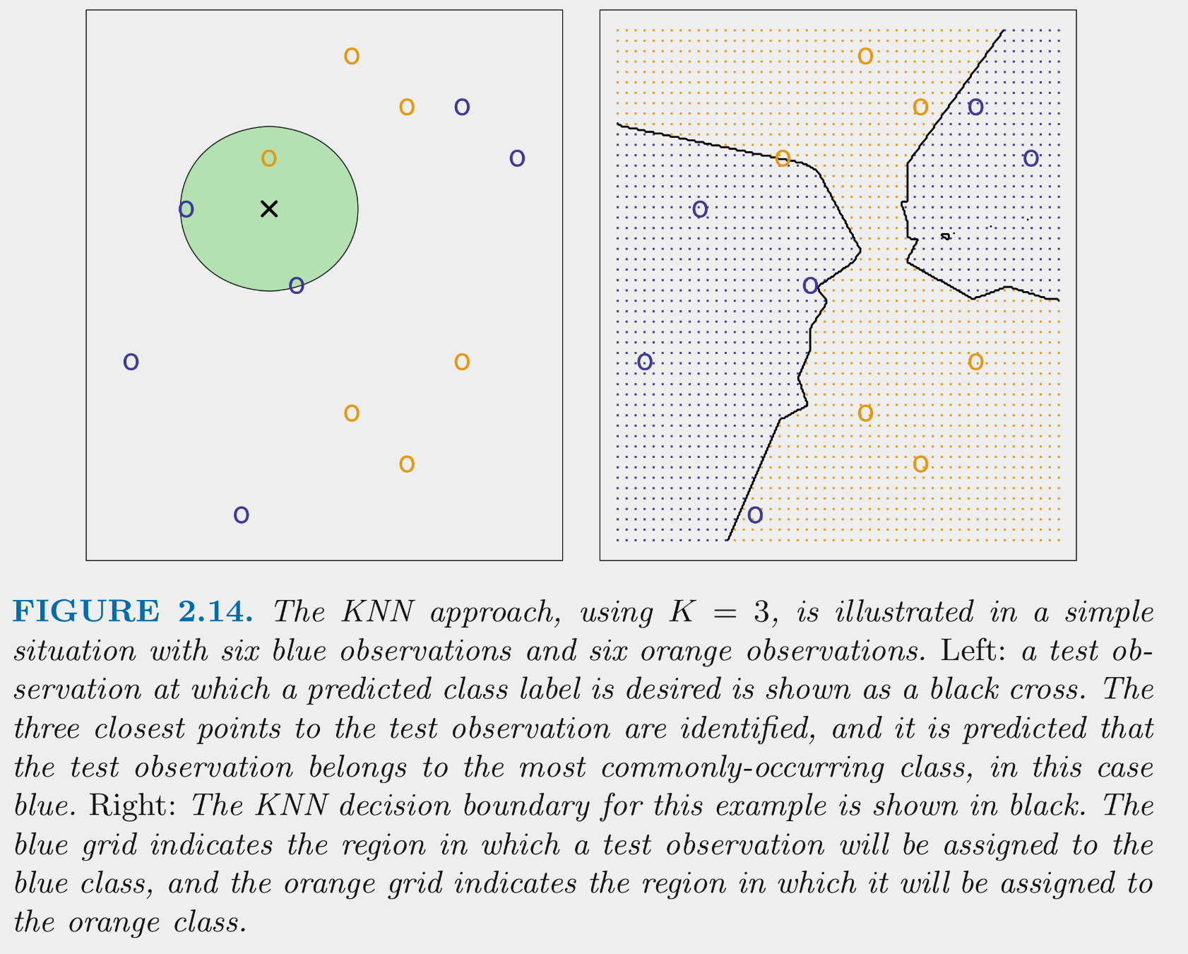
The above figure illustrates the application of 3-NN to a small sample training set (N = 12) with 2 predictors
- For test observation X in the left panel, we would predict class = blue because blue is the majority class (highest probability) among the 3 nearest training observations
- If we calculated these probabilities for all possible combinations of the two predictors in the training set, it would yield the decision boundaries depicted in the right panel
KNN can produce complex decision boundaries
- This makes it flexible (can reduce bias)
- This makes it susceptible to variance problems
How do we handle this bias-variance trade-off for KNN classification?
- Choose the appropriate value for K. As K increases, variance reduces (but bias may increase). As K decreases, bias may be reduced but variance increases. Choose a K that produces good performance in test data.
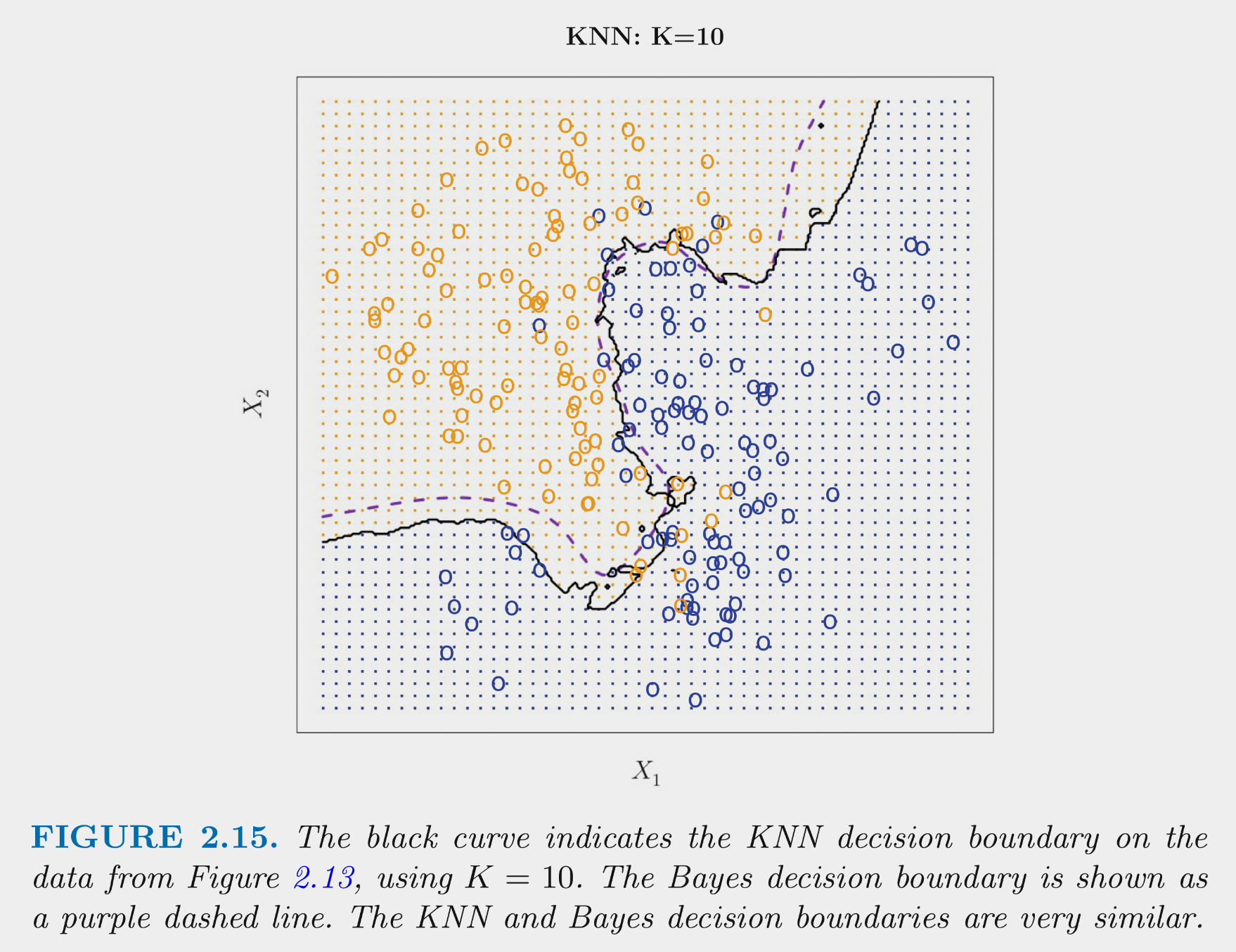
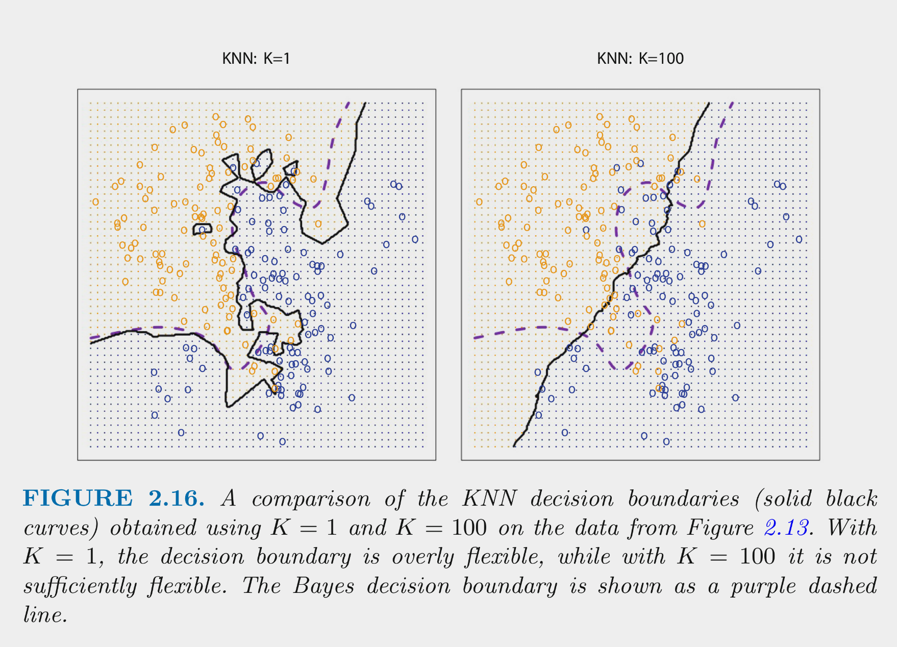
These figures depict the KNN (and Bayes classifier) decision boundaries for the earlier simulated 2 class problem with \(X_1\) and \(X_2\)
- K = 10 appears to provide the sweet spot b/c it closely approximates the Bayes decision boundary
- Of course, you wouldnt know the true Bayes decision boundary if the data were real (not simulated)
- But K = 10 would also yield the lowest test error (which is how it should be chosen)
- Bayes classifier test error: .1304
- K = 10 test error: 1363
- K = 1 test error: .1695
- K = 100 test err: .1925
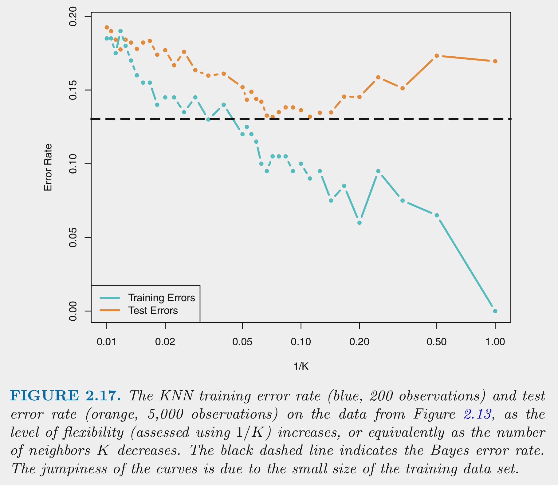
You can NOT make the decision about K based on training error
This figure depicts training and test error for simulated data example as function of 1/K
Training error decreases as 1/K increases. At 1 (K=1) training error is 0
Test error shows expected inverted U
- For high K (left side), error is high because of high variance
- As move right (lower K), variance is reduced rapidly with little increase in bias. Error is reduced.
- Eventually, there is diminishing return from reducing variance but bias starts to increase rapidly. Error increases again.
Lets demonstrate KNN using the Auto dataset
- Load fresh copy of dataset
- Add dummy variables
- Split again into training and test
auto <- as_tibble(Auto) %>%
  mutate(high_mpg = if_else(mpg > median(mpg),1,0), #make a high/low mpg variable to demo classification
         high_mpg = factor(high_mpg, levels = c(0,1), labels = c("low", "high"))) %>%
  select(-mpg, - name) %>%
  mutate(origin = as.factor(origin))

dmy_codes <- dummyVars(~origin, sep = "_", fullRank = TRUE,
                       data = auto)
dmy_data <- as_tibble(predict(dmy_codes, auto))
auto <- auto %>%
  bind_cols (dmy_data) %>%
  select(-origin) %>%
  select(high_mpg, everything())


set.seed(20110522)
auto_splits <- initial_split(auto, prop = .75, strata = "high_mpg")
trn <- training(auto_splits)
test <- testing(auto_splits)
Normalize the predictors
## Created from 294 samples and 9 variables
##
## Pre-processing:
##   - ignored (1)
## - re-scaling to [0, 1] (8)## Observations: 294
## Variables: 9
## $ high_mpg <fct> low, low, low, low, low, low, low, low, low, low, high, low, low, h…
## $ cylinders <dbl> 1.0, 1.0, 1.0, 1.0, 1.0, 1.0, 1.0, 1.0, 1.0, 1.0, 0.2, 0.6, 0.6, 0.…
## $ displacement <dbl> 0.72868217, 0.64599483, 0.60465116, 0.93281654, 0.96124031, 1.00000…
## $ horsepower <dbl> 0.6467391, 0.5652174, 0.5108696, 0.8260870, 0.9184783, 0.9728261, 0…
## $ weight <dbl> 0.61465721, 0.53871158, 0.54255319, 0.80614657, 0.79757683, 0.83096…
## $ acceleration <dbl> 0.20833333, 0.17857143, 0.14880952, 0.11904762, 0.02976190, 0.11904…
## $ year <dbl> 0.00000000, 0.00000000, 0.00000000, 0.00000000, 0.00000000, 0.00000…
## $ origin_2 <dbl> 0, 0, 0, 0, 0, 0, 0, 0, 0, 0, 0, 0, 0, 0, 1, 1, 1, 1, 1, 0, 0, 0, 0…
## $ origin_3 <dbl> 0, 0, 0, 0, 0, 0, 0, 0, 0, 0, 1, 0, 0, 1, 0, 0, 0, 0, 0, 0, 0, 0, 0…## Observations: 98
## Variables: 9
## $ high_mpg <fct> low, low, low, low, low, low, low, low, low, low, low, high, high, …
## $ cylinders <dbl> 1.0, 1.0, 1.0, 1.0, 0.6, 1.0, 1.0, 1.0, 1.0, 0.6, 0.6, 0.2, 0.2, 0.…
## $ displacement <dbl> 0.617571059, 0.609819121, 0.997416021, 0.813953488, 0.335917313, 0.…
## $ horsepower <dbl> 0.4565217, 0.5652174, 0.9456522, 0.6739130, 0.2663043, 0.9184783, 0…
## $ weight <dbl> 0.55880615, 0.53782506, 0.80998818, 0.57624113, 0.36052009, 0.88711…
## $ acceleration <dbl> 0.23809524, 0.23809524, 0.05952381, 0.11904762, 0.44642857, 0.35714…
## $ year <dbl> 0.00000000, 0.00000000, 0.00000000, 0.00000000, 0.00000000, 0.00000…
## $ origin_2 <dbl> 0, 0, 0, 0, 0, 0, 0, 0, 0, 0, 0, 1, 0, 0, 0, 0, 0, 0, 0, 1, 0, 0, 0…
## $ origin_3 <dbl> 0, 0, 0, 0, 0, 0, 0, 0, 0, 0, 0, 0, 1, 0, 1, 0, 0, 0, 0, 0, 0, 0, 0…Train some models using two predictors and varying k
Save training and test accuracies in \(acc\) tibble
acc <-tibble(k = numeric(), acc_train = numeric(), acc_test = numeric())

k_values = c(1,5,10,20,50)

for (k in k_values) {
  knn <- train(high_mpg ~ displacement + year, data = trn_norm,
            method = "knn", trControl = trn_ctrl, tuneGrid = tibble(k = k))

  acc <- bind_rows(acc, tibble(k=k,
                               acc_train = accuracy(predict(knn, trn_norm), trn_norm$high_mpg),
                               acc_test = accuracy(predict(knn, test_norm), test_norm$high_mpg)))
}
Looks like the best model is k = 10
| k | acc_train | acc_test |
|---|---|---|
| 1 | 0.9863946 | 0.9183673 |
| 5 | 0.9285714 | 0.9081633 |
| 10 | 0.9115646 | 0.9285714 |
| 20 | 0.8979592 | 0.8979592 |
| 50 | 0.8979592 | 0.8877551 |
Lets look at the decision boundaries for 10-NN in training and test
- Fit the 10-NN model in training
knn10 <- train(high_mpg ~ displacement + year, data = trn_norm,
            method = "knn", trControl = trn_ctrl, tuneGrid = tibble(k = 10))
Plot decision boundaries:
- Training
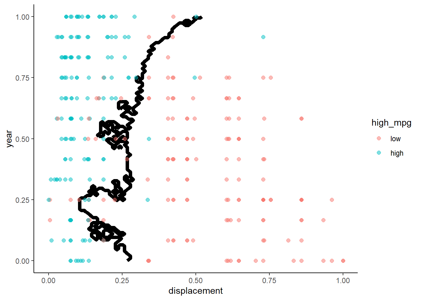
- Test
What are your thoughts about the use of GLM vs. KNN for understanding the factors that predict high_mpg?
- GLM provides coefficients (parameter estimates) that can be used to describe changes in probability, odds and odds ratio associated with change for any x. These parameter estimates can be tested via inferential procedures. KNN does not provide any of this. With KNN, we can visualize decision boundary or predicted Y by any x, controlling for other x but these relationships may be complex in shape.
What would you have to do to display the relationship between displacement and high_mpg?
- You could plot of ‘probability’ of high_mpg by displacement, holding year constant at its mean based on 10-NN.
Plot of “probability” of high_mpg by displacement, holding year constant at its mean based on 10-NN
- Generate values of displacement across range to display
- Set year = mean year
- Normalize using training set values
- Predict probabilities using 10-NN fit to training set
pred_data <- tibble(displacement = seq(min(trn$displacement), max(trn$displacement), length = 200),
                    year = mean(trn$year),
                    acceleration = NA,
                    cylinders = NA,
                    horsepower = NA,
                    weight = NA,
                    origin_2 = NA,
                    origin_3 = NA)

pred_data_norm <- predict(normalize, pred_data)
pred_data$pr_pred <- predict(knn10, pred_data_norm, "prob")$high #put predictions back into data file with raw units

ggplot(data=pred_data, aes(displacement, pr_pred)) +
  geom_line(color = "red") +
  geom_point(data=trn, aes(displacement, as.numeric(high_mpg) - 1), position = position_jitter(height = 0.03, width = 0)) +
labs(x = "Displacement", y = "Pr(High MPG | Displacement)") 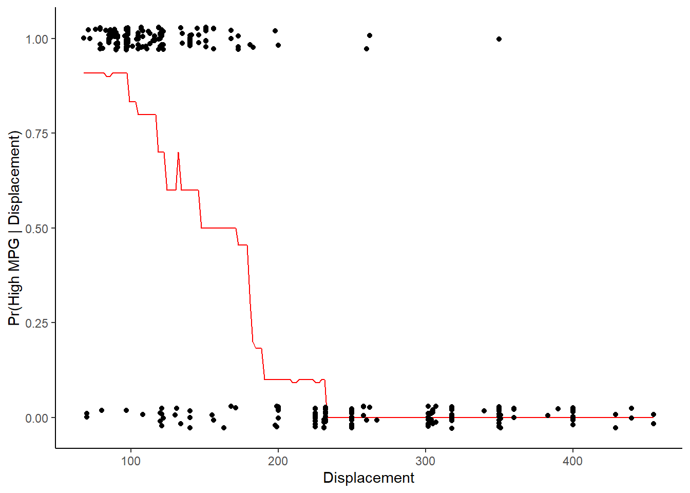
3.5 Linear discriminant analysis
LDA models the distributions of the Xs separately for each class
Then uses Bayes theorem to estimate $Pr(Y = k | X) for each k and assigns the observation to the class with the highest probability
\[Pr(Y = k|X) = \frac{\pi_k * f_k(X)}{\sum_{l = 1}^{K} f_l(X)}\]
where
- \(\pi_k\) is the prior probability that an observation comes from class k (estimated from frequencies of k in training)
- \(f_k(X)\) is the density function of X for an observation from class k
- \(f_k(X)\) is large if there is a high probability that an observation in class k has that set of values for X and small if that probability is low
- \(f_k(X)\) is difficult to estimate unless we make some simplifying assumptions (i.e., X is multivariate normal and common covariance matrix (\(\sum\)) across K classes)
- With these assumptions, we can estimate \(\pi_k\), \(\mu_k\), and \(\sigma^2\) from the training set and calculate \(Pr(Y = k|X)\) for each k
With a single predictor, the probability of any class k, given X is:
\[Pr(Y = k|X) = \frac{\pi_k \frac{1}{\sqrt{2\pi\sigma}}\exp(-\frac{1}{2\sigma^2}(x-\mu_k)^2)}{\sum_{l=1}^{K}\pi_l\frac{1}{2\sigma^2}\exp(-\frac{1}{2\sigma^2}(x-\mu_l)^2)}\]
LDA is a parametric model, but is it interpretable?
Application of LDA to Auto data set with two predictors
Notice that LDA produces linear decision boundary (see James et al. (2013) for formula for discriminant function derived from the probability function on last slide)
lda <- train(high_mpg ~ displacement + year, data = trn,
            method = "lda", trControl = trn_ctrl)

accuracy(predict(lda, test), test$high_mpg)
## [1] 0.877551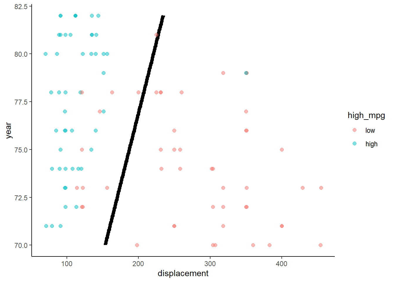
3.6 Quadratic discriminant analysis
QDA relaxes one restrictive assumption of LDA
- Still required multivariate normal X
- But it allows each class to have its own \(\sum\)
- This makes it:
- More flexible
- Able to model non-linear decision boundaries (see formula for discriminant in James et al. (2013))
- But requires substantial increase in parameter estimation (more potential to overfit)
Application of QDA to Auto data set with two predictors
qda <- train(high_mpg ~ displacement + year, data = trn,
            method = "qda", trControl = trn_ctrl)

accuracy(predict(qda, test), test$high_mpg)
## [1] 0.8979592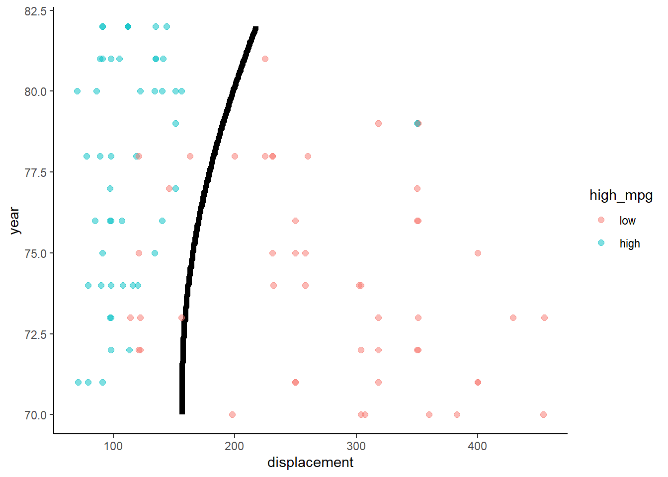
3.7 Comparisons between these four classifiers
Both logistic and LDA are linear functions of X and therefore produce linear decision boundaries
LDA makes additional assumptions about X (multivariate normal and common \(\sum\)) beyond logistic regression. Relative performance is based on the quality of this assumption
QDA relaxes the LDA assumption about common \(\sum\).
- This also allows for nonlinear decision boundaries
- QDA is therefore more flexible, which means possibly less bias but more potential for overfitting
Both QDA and LDA assume multivariate normal X so may not accommodate categorical predictors very well. Logistic and KNN do
KNN is non-parametric and therefore the most flexible
- Increased overfitting, decreased bias?
- Not very interpretable. But LDA/QDA, although parametric, arent as interpretable as logistic regression
Logistic regression fails when classes are perfectly separated (but does that ever happen?) and is less stable when classes are well separated
LDA, KNN, and QDA naturally accommodate more than two classes
- Logistic requires additional tweak (Briefly describe: multiple one vs other classes models approach)
3.8 A quick tour of many classifiers
The Auto dataset had strong predictors and a mostly linear decision boundary for the two predictors we considered
This will not be true in many cases
Lets consider a more complex two predictor decision boundary in the circle dataset from the \(mlbench\) package (lots of cool datasets for ML)
Adapted to caret from a demonstration by Michael Hahsler
library(mlbench)
set.seed(20140102)
trn <- as_tibble(mlbench.circle(200)) %>%
  rename(x1 = x.1, x2 = x.2) %>%
  glimpse()
## Observations: 200
## Variables: 3
## $ x1 <dbl> -0.514721263, 0.763312056, 0.312073042, 0.162981535, -0.320294696, -0.37…
## $ x2 <dbl> 0.47513532, 0.65803777, -0.89824011, 0.38680494, -0.47313964, 0.56086402…
## $ classes <fct> 1, 2, 2, 1, 1, 1, 1, 2, 2, 1, 2, 2, 1, 1, 1, 2, 2, 2, 2, 2, 2, 2, 2, 2, …test <- as_tibble(mlbench.circle(200)) %>%
rename(x1 = x.1, x2 = x.2)
ggplot(data=trn, aes(x = x1, y = x2, color = classes)) +
geom_point(size = 2, alpha = .5)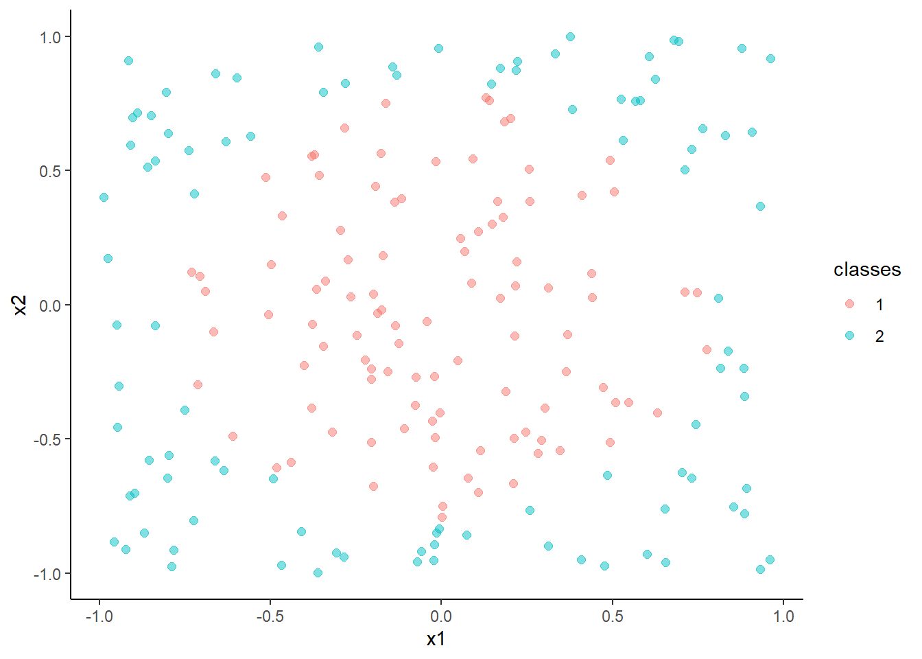
- Logistic Regression
m <- train(classes ~ x1 + x2, data = trn, method = "glm", family = "binomial",
              trControl = trn_ctrl)

accuracy(predict(m, test, "raw"), test$classes )
## [1] 0.62
Now lets fit a series of classifiers to train and then look at decision boundaries in test
- KNN (k = 1)
m <- train(classes ~ x1 + x2, data = trn, method = "knn",
              trControl = trn_ctrl, tuneGrid = tibble(k = 1))

accuracy(predict(m, test, "raw"), test$classes )
## [1] 0.975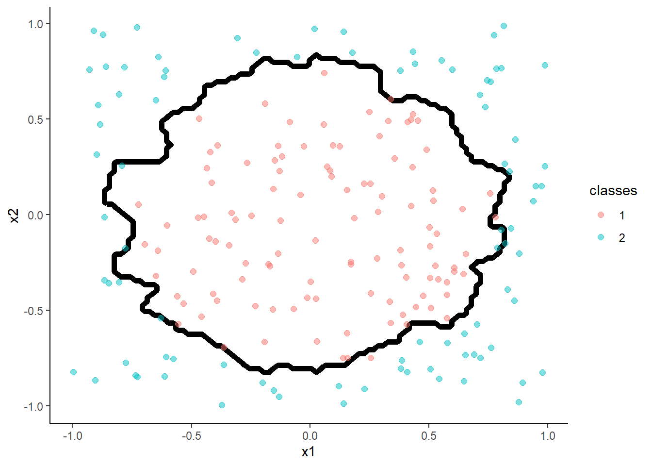
- Linear Discriminant Analysis
m <- train(classes ~ x1 + x2, data = trn, method = "lda",
              trControl = trn_ctrl)

accuracy(predict(m, test, "raw"), test$classes )
## [1] 0.62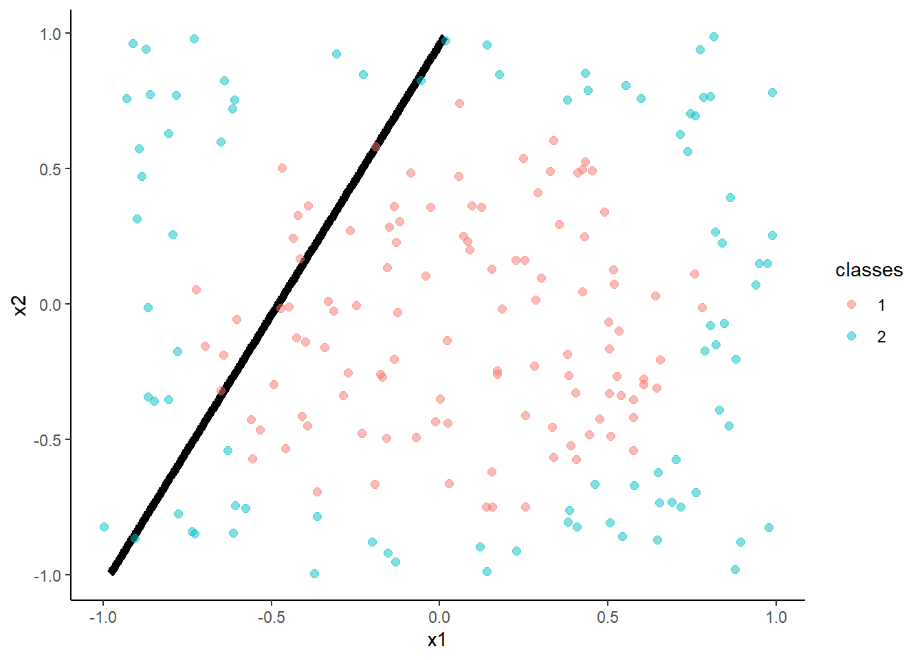
- Quadratic Discriminant Analysis
m <- train(classes ~ x1 + x2, data = trn, method = "qda",
              trControl = trn_ctrl)

accuracy(predict(m, test, "raw"), test$classes )
## [1] 0.93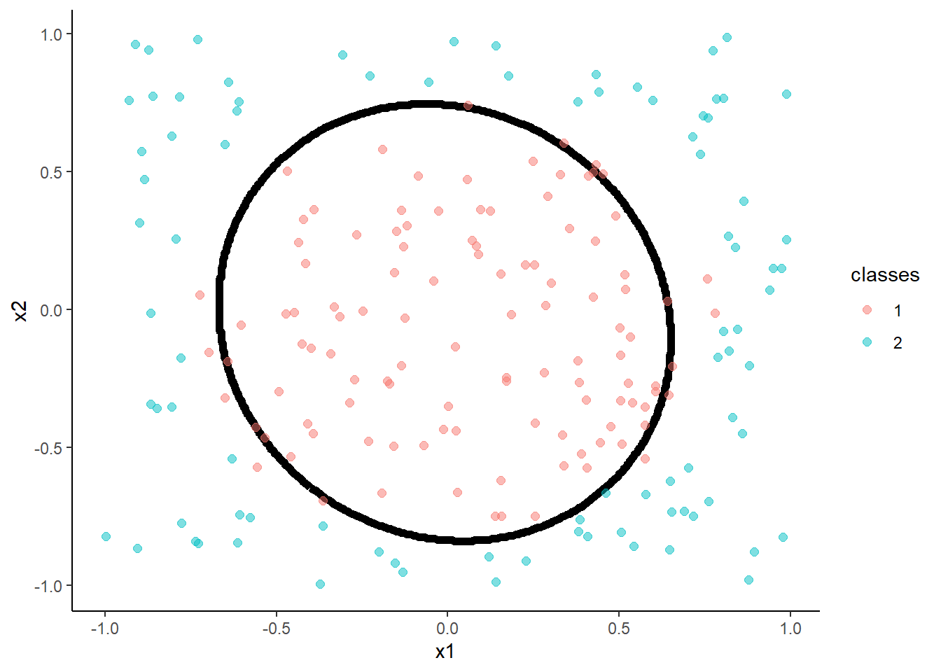
Naive Bayes Classifier
- The Naïve Bayes classifier is a simple probabilistic classifier which is based on Bayes theorem
- But, we assume that the predictor variables are conditionally independent of one another given the response value
- There are many tutorials available on this classifier
m <- train(classes ~ x1 + x2, data = trn, method = "nb",
           trControl = trn_ctrl,
           tuneGrid = tibble(fL = 0, usekernel = TRUE, adjust = 1))

accuracy(predict(m, test, "raw"), test$classes )
## [1] 0.99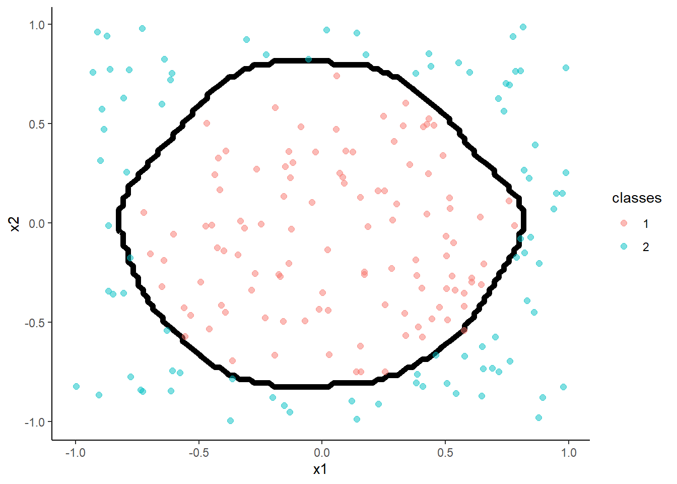
Random Forest
- Random Forest is a variant of decision trees
- It uses bagging which involves resampling the data to produce many trees and then aggregating across trees for the final classification
m <- train(classes ~ x1 + x2, data = trn,
           method = "rf", tuneGrid = tibble(mtry = 2), n.trees = 500,
           trControl = trn_ctrl)

accuracy(predict(m, test, "raw"), test$classes )
## [1] 0.975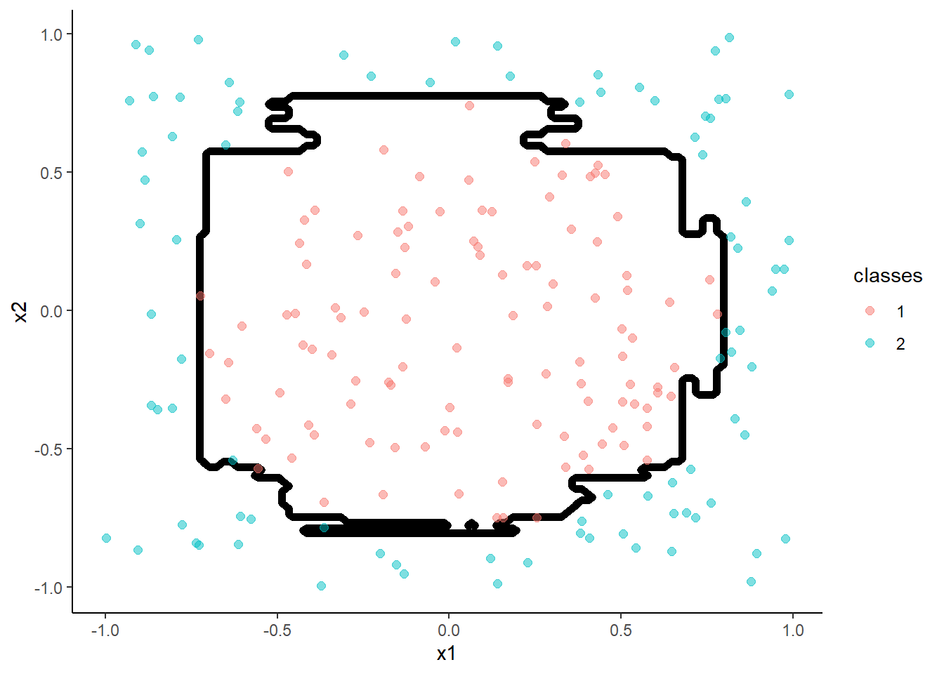
- Support Vector Machine
- Incorporates kernels (transformations of x) directly into the algorithm
- Linear kernal (not displayed) similar to logistic regression
- Other kernels useful for non-linear effects
Here is a polynomial kernel
m <- train(classes ~ x1 + x2, data = trn,
           method = "svmPoly", tuneLength = 3)

m <- train(classes ~ x1 + x2, data = trn,
           method = "svmPoly", tuneGrid = tibble(degree = 3, scale = 0.1, C = 1),
           trControl = trn_ctrl)

accuracy(predict(m, test, "raw"), test$classes )
## [1] 0.99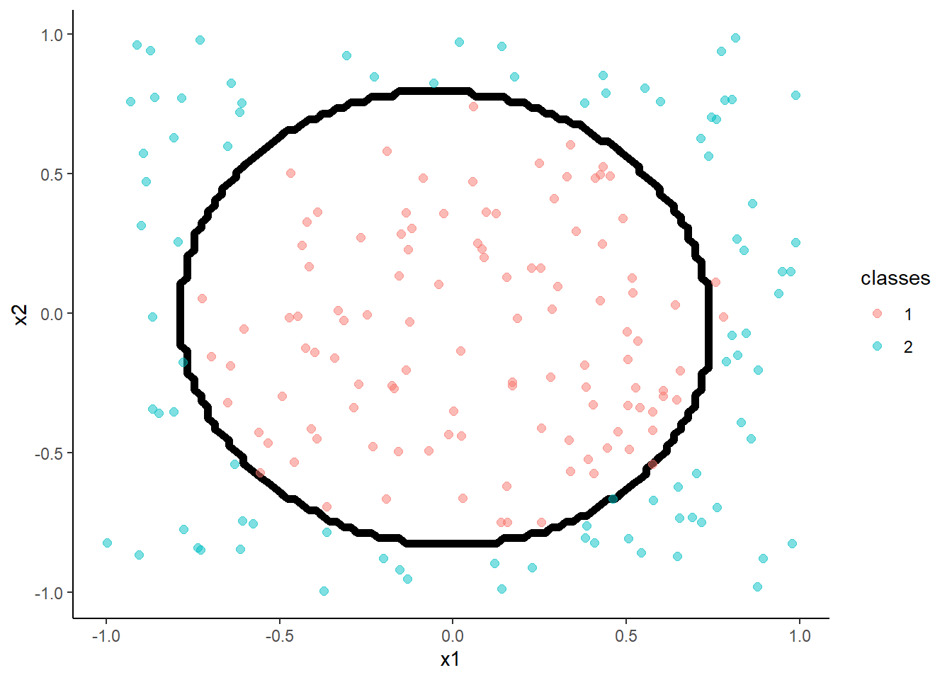
- SVM with Radial Basis Function Kernel
m <- train(classes ~ x1 + x2, data = trn,
           method = "svmRadial", tuneLength = 4)

m <- train(classes ~ x1 + x2, data = trn,
           method = "svmRadial", tuneGrid = tibble(C = 2, sigma = 0.7751589),
           trControl = trn_ctrl)

accuracy(predict(m, test, "raw"), test$classes )
## [1] 0.975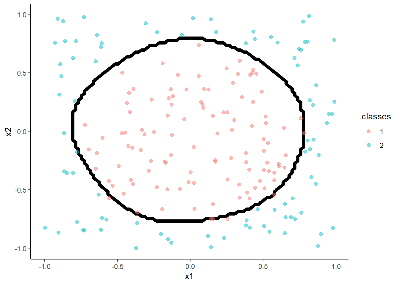
- Feed-forward neural networks with a single hidden layer
With 1 hidden unit:
m <- train(classes ~ x1 + x2, data = trn,
           method = "nnet", tuneGrid = tibble(size = 1, decay = 0.003162278),
           trControl = trn_ctrl)
## # weights: 5
## initial value 147.399058
## iter 10 value 135.581487
## iter 20 value 120.511937
## iter 30 value 120.285463
## final value 120.285456
## converged## [1] 0.67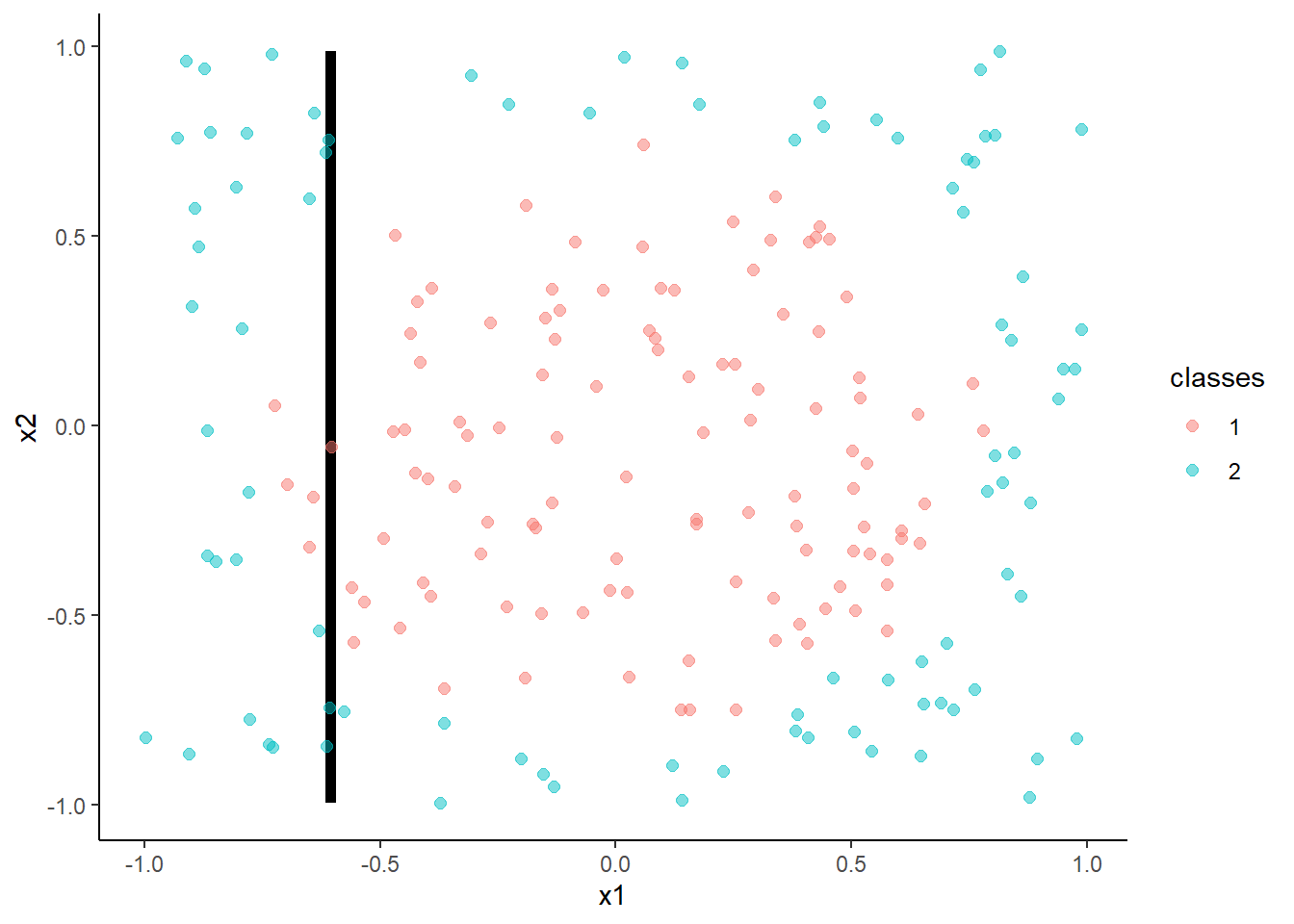
- Feed-forward neural networks with a single hidden layer
With 2 hidden units:
m <- train(classes ~ x1 + x2, data = trn,
           method = "nnet", tuneGrid = tibble(size = 2, decay = 0.003162278),
           trControl = trn_ctrl)
## # weights: 9
## initial value 152.774764
## iter 10 value 116.764443
## iter 20 value 100.212536
## iter 30 value 98.533875
## iter 40 value 88.376463
## iter 50 value 85.975247
## iter 60 value 85.835023
## iter 70 value 85.812816
## final value 85.812698
## converged## [1] 0.815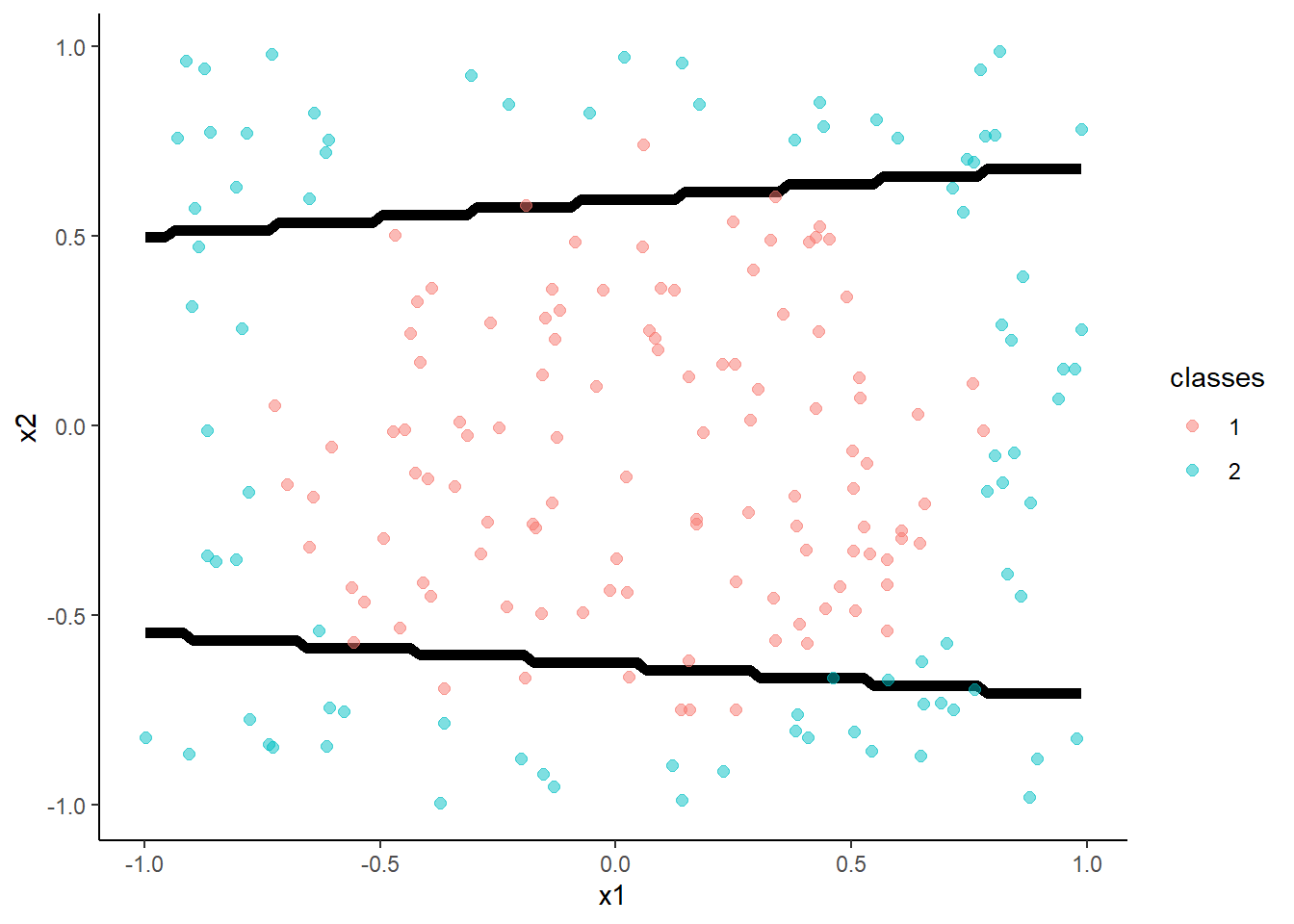
- Feed-forward neural networks with a single hidden layer
With 5 hidden units:
m <- train(classes ~ x1 + x2, data = trn,
           method = "nnet", tuneGrid = tibble(size = 5, decay = 0.003162278),
           trControl = trn_ctrl)
## # weights: 21
## initial value 150.231536
## iter 10 value 107.608962
## iter 20 value 48.203415
## iter 30 value 27.382335
## iter 40 value 21.034676
## iter 50 value 19.390978
## iter 60 value 17.211395
## iter 70 value 15.927442
## iter 80 value 15.697463
## iter 90 value 15.679830
## iter 100 value 15.675472
## final value 15.675472
## stopped after 100 iterations## [1] 0.97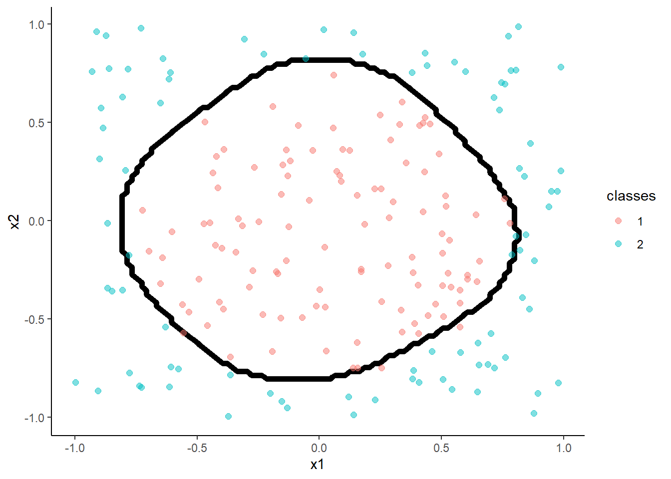
3.9 Classification model performance metrics
There are MANY common metrics and methods for evaluating the performance of a classification model. This include:
- Confusion matrices
- Accuracy
- Sensitivity, specificity, positive and negative predictive value (PPV, NPV) [see also: precision/recall]
- Balanced accuracy & F1
- Kappa
- Receiver operating characteristic (ROC) curve and area under the curve (AUC) [see also: PR curve and prAUC]
The best metric/method is a function both of your intended use and the class distributions
For example, accuracy is widely understood but can be misleading when class distributions are highly unbalanced
Sensitivity/Specificity are common in literatures that consider diagnosis (clinical psychology/psychiatry, medicine)
Positive/Negative predictive value are key to consider with sensitivity/specificity when classes are unbalanced
ROC curve and AUC provide nice summary visualization and metric when considering thresholds other than 50% (also common when classes are unbalanced or types of errors matter)
We will consider examples of these metrics/methods in balanced (Auto) and unbalanced (credit card default) situations after some general definitions
The Confusion Matrix
| Reference | ||
|---|---|---|
| Prediction | Negative | Positive |
| Negative | TN | FN |
| Positive | FP | TP |
Definitions:
TN - True negative
TP - True positive
FP - False positive (Type 1 error/false alarm)
FN - False negative (Type 2 error/miss)
Perfect classifier has all the observations on the diagonal
The two types of errors may have different costs (more in a moment)
Defining common metrics from Confusion Matrix:
| Reference | ||
|---|---|---|
| Prediction | Negative | Positive |
| Negative | TN | FN |
| Positive | FP | TP |
\(Accuracy = \frac{TN + TP}{TN + TP + FN + FP}\)
\(Sensitivity\:(Recall) = \frac{TP}{TP + FN}\)
\(Specificity = \frac{TN}{TN + FP}\)
\(Positive\:Predictive\:Value\:(Precision) = \frac{TP}{TP + FP}\)
\(Negative\:Predictive\:Value = \frac{TN}{TN + FN}\)
\(Balanced\:accuracy = \frac{Sensitivity + Specificity}{2}\)
\(F_\beta\) score:
\(F1 = 2 * \frac{Precision * Recall}{Precision + Recall}\) (most common; harmonic mean of precision and recall)
\(F_\beta = (1 + \beta^2) * \frac{Precision * Recall}{(\beta^2*Precision) + Recall}\)
\(F_\beta\) was derived so that it measures the effectiveness of a classifier for someone who assigns \(\beta\) times as much importance to recall as precision
A balanced example:
Two predictor logistic regression in Auto data set
Can get these metrics using caret’s \(confusionMatrix()\)
Should specify positive class label (otherwise, caret assumes the first level is positive)
Should be done in test of course!
## Confusion Matrix and Statistics
##
##           Reference
## Prediction low high
##       low   41    1
##       high   8   48
##
##                Accuracy : 0.9082
##                  95% CI : (0.8328, 0.9571)
##     No Information Rate : 0.5
##     P-Value [Acc > NIR] : <2e-16
##
##                   Kappa : 0.8163
##
##  Mcnemar's Test P-Value : 0.0455
##
##             Sensitivity : 0.9796
##             Specificity : 0.8367
##          Pos Pred Value : 0.8571
##          Neg Pred Value : 0.9762
##              Prevalence : 0.5000
##          Detection Rate : 0.4898
##    Detection Prevalence : 0.5714
##       Balanced Accuracy : 0.9082
##
##        'Positive' Class : high
##
An unbalanced example with 50% threshold
- LDA classifier used to predict credit card default (yes vs. no) with 50% (Bayes classifier) threshold from James et al. (2013)
## Confusion Matrix and Statistics
##
##           Reference
## Prediction   No  Yes
##        No  9644  252
##        Yes   23   81
##
##                Accuracy : 0.9725
##                  95% CI : (0.9691, 0.9756)
##     No Information Rate : 0.9667
##     P-Value [Acc > NIR] : 0.0004973
##
##                   Kappa : 0.3606
##
##  Mcnemar's Test P-Value : < 2.2e-16
##
##             Sensitivity : 0.2432
##             Specificity : 0.9976
##          Pos Pred Value : 0.7788
##          Neg Pred Value : 0.9745
##              Prevalence : 0.0333
##          Detection Rate : 0.0081
##    Detection Prevalence : 0.0104
##       Balanced Accuracy : 0.6204
##
##        'Positive' Class : Yes
##
How can we improve sensitivity (recall)?
- We can use a more liberal/lower threshold for saying someone will default. For example, rather than requiring a 50% probability to classify as yes for default, we could lower to 20% threshold
What will the consequences of this change be?
- First, the Bayes classifier threshold of 50% produces the highest overall accuracy so accuracy will drop. If we think about this change as it applies to the columns of our confusion matrix, we will now catch more of the defaults (fewer false negatives/misses), so sensitivity will go up. This was the goal of the lower threshold. However, we will also end up with more false positives so specificity will drop. If you consider the rows of the confusion matrix, we will have more false positives so the PPV will drop. However, we will have fewer false negatives so the NPV will increase. Whether these trade-offs are worth it are a function of the cost of different types of errors and how much you gain and lose with regard to each type of performance metric (ROC can inform this; more in a moment)
An unbalanced example with 20% threshold
- LDA classifier used to predict credit card default (yes vs. no) with 20% threshold from James et al. (2013)
## Confusion Matrix and Statistics
##
##           Reference
## Prediction   No  Yes
##        No  9432  138
##        Yes  235  195
##
##                Accuracy : 0.9627
##                  95% CI : (0.9588, 0.9663)
##     No Information Rate : 0.9667
##     P-Value [Acc > NIR] : 0.9869
##
##                   Kappa : 0.4921
##
##  Mcnemar's Test P-Value : 6.671e-07
##
##             Sensitivity : 0.5856
##             Specificity : 0.9757
##          Pos Pred Value : 0.4535
##          Neg Pred Value : 0.9856
##              Prevalence : 0.0333
##          Detection Rate : 0.0195
##    Detection Prevalence : 0.0430
##       Balanced Accuracy : 0.7806
##
##        'Positive' Class : Yes
##
You can begin to visualize the classifier performance by threshold simply by plotting histograms of the predicted positive class probabilities, separately for the true positive and negative classes
Ideally, the probabilities mostly low for the true negative class and mostly high for the true positive class
Here is this plot for the two predictor logistic regression for auto dataset
ggplot(data = test, aes(x = predict(lr1,test, "prob")$high)) +
  geom_histogram() +
  facet_wrap(~high_mpg) +
  xlab("Pr(High MPG)")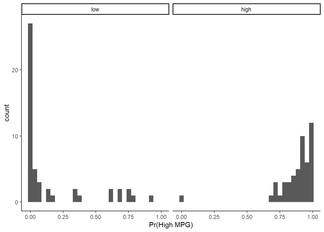
You could also do this in train to begin to identify cases which are mis-classified as part of exploring for additional predictors
The Receiver Operating Characteristics (ROC) curve for a classifier provides a more formal method to visualize the trade-offs between Sensitivity and Specificity across all possible thresholds for classification.
Lets look at this in the context of the logistic regression classifier for auto
- Will use \(roc.curve()\) from \(PRROC\) library
- Predictions input as \(scores.class0\). Use probabilities for positive class.
- Reference/labels input as \(weights.class0\)
- For weights, positive class = 1 , negative class = 0
library(PRROC)
roc <- roc.curve(scores.class0 = predict(lr1, test, "prob")$high, weights.class0 = as.numeric(test$high_mpg)-1, curve = TRUE)
ROC object includes:
- The area under the ROC curve
- The raw data to plot the ROC curve (columns are false-positive rate, sensitivity, and threshold, respectively)
## [1] "type" "auc" "curve"## [1] 0.9737609## [,1] [,2] [,3]
## [1,] 0 0.00000000 0.9909287
## [2,] 0 0.02040816 0.9891691
## [3,] 0 0.06122449 0.9865586
## [4,] 0 0.08163265 0.9855625
## [5,] 0 0.10204082 0.9839133
## [6,] 0 0.12244898 0.9814696ROC also has plot method to display directly
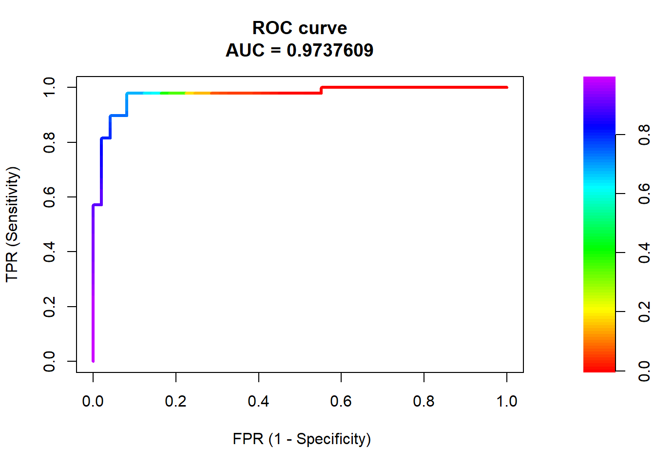
Random classifier would have a diagonal curve from bottom-left to top-right
Perfect classifier would reach up to top-left corner (TPR = 1 at FPR = 0)
Area under the ROC curve (AUC):
Ranges from 1.0 (perfect) down to approximately 0.5 (random classifier)
- If the AUC was consistently less than 0.5, then the predictions could simply be inverted
AUC is the probability that the classifier will rank/predict a randomly selected true positive observation higher than a randomly selected true negative observation
AUC is a very common classification metric because it summarizes performance across all possible thresholds
AUC is not affected by class imbalances (vs. Area under the precision-recall curve; not discussed)

Cohen’s Kappa
There is a great explanation of kappa on stack overflow
Wikipedia also has a very detailed definition and explanation as well (though not in the context of machine learning)
Compares observed accuracy to expected accuracy (random chance)
\(Kappa = \frac{observed\:accuracy - expected\:accuracy}{1 - expected\:accuracy}\)
When outcome is unbalanced, some agreement/accuracy (relationship between model predictions and reference/ground truth) is expected
Kappa adjusts for this
Kappa is essentially the proportional increase in accuracy above the accuracy expected by the base rates of the reference and classifier
To calculate the expected accuracy, we need to consider the probabilities of reference and classifier prediction both being positive (and both being negative) by chance given the base rates of these classes for the reference and classifier.
| Reference | ||
|---|---|---|
| Prediction | Negative | Positive |
| Negative | A | B |
| Positive | C | D |
\(P_{positive} = \frac{B + D}{A + B + C + D} * \frac{C + D}{A + B + C + D}\)
\(P_{negative} = \frac{A + C}{A + B + C + D} * \frac{A + B}{A + B + C + D}\)
\(P_{expected} = P_{positive} + P_{negative}\)
Returning to the unbalanced credit default example
## Confusion Matrix and Statistics
##
##           Reference
## Prediction   No  Yes
##        No  9667  229
##        Yes    0  104
##
##                Accuracy : 0.9771
##                  95% CI : (0.974, 0.9799)
##     No Information Rate : 0.9667
##     P-Value [Acc > NIR] : 5.515e-10
##
##                   Kappa : 0.4675
##
##  Mcnemar's Test P-Value : < 2.2e-16
##
##             Sensitivity : 0.3123
##             Specificity : 1.0000
##          Pos Pred Value : 1.0000
##          Neg Pred Value : 0.9769
##              Prevalence : 0.0333
##          Detection Rate : 0.0104
##    Detection Prevalence : 0.0104
##       Balanced Accuracy : 0.6562
##
##        'Positive' Class : Yes
##
\(P_{positive} = \frac{229 + 104}{10000} * \frac{0 + 104}{10000} = .0003\)
\(P_{negative} = \frac{9667 + 0}{10000} * \frac{9667 + 229}{1000} = .9566\)
\(P_{expected} = .0003 + .9566 = .9569\)
\(Accuracy = .9771\)
\(Kappa = \frac{observed\:accuracy - expected\:accuracy}{1 - expected\:accuracy}\)
\(Kappa = \frac{.9771 - .9569}{1 - .9569} = .47\)
Kappa Rules of Thumb w/ a big grain of salt…….
- Kappa < 0: No agreement
- Kappa between 0.00 and 0.20: Slight agreement
- Kappa between 0.21 and 0.40: Fair agreement
- Kappa between 0.41 and 0.60: Moderate agreement
- Kappa between 0.61 and 0.80: Substantial agreement
- Kappa between 0.81 and 1.00: Almost perfect agreement.