1 Overview of Machine Learning Concepts and Uses
This unit will provide:
- A course overview, structure, expectations, etc
- A discussion of Yarkoni and Westfall (2017)
- Introduction of key concepts and definitions including:
- Useful framework for machine learning
- Details on supervised techniques
- Estimating \(f\), the true data generating process
- Assessing model performance
- An empirical demonstration of the Bias-Variance trade off
1.1 Course Overview
- Introductions (preferred name, pronouns, year in program, lab/area, prior experiences/comfort with R and machine learning)
- Syllabus review
- Reading assignments
- Homework assignments
- Course as guided learning
- Lecture is discussion oriented
- Learning by doing
- Use of “Tidy style” is expected
- Need to learn data wrangling and programing (will focus on tidyverse)
- R Markdown is key tool (course notes and slides make with superset of Markdown- bookdown and revealjs)
- This is “beta” release of course that will eventually be required for data science masters
- Course timeline/lecture pace will be flexible to meet your needs (as I learn them)
- Course uses power lecture format with 15 mins of post-class office hours/lab
- Why R?
- Why me?
1.2 Discussion of Yarkoni 2017
This section abstracts key points (often verbatim) from the paper to discuss in class
1.2.1 Goal of scientific psychology is to understand human behavior
Involves both explaining behavior (i.e., identifying causes) and predicting (yet to be observed) behaviors
Explanation and prediction are often in conflict
- Model of data-generating process may not provide best prediction - too complex?
- Psychological phenomena may be too complex to represent in models that are comprehensible to us
- Models we can understand may account for too little variance for precise prediction
Ideal explanatory science is not generally ideal predictive science, and vice versa
Scientists may have to choose between:
- Developing complex models that can accurately predict outcomes of interest but fail to respect known psychological or neurobiological constraints
- Building simple models that appear theoretically elegant but have very limited capacity to predict actual human behavior.
Yarkoni and Westfall (2017) claim (and Curtin agrees) that research programs that emphasize prediction (and that treat explanation as a secondary goal) may be more fruitful both in the short-term and the long-term.
Machine learning combined with large(?) datasets including human behavior now make this possible
What is the value of black box predictive models? Examples?
- Prediction models can both serve important applications and test theories. For example, temporally precise prediction of suicide attempts or relapse aid simply ‘just-in-time’ intervention efforts. Precision medicine/mental health requires predicting what treatment works best for who (and when). Prediction models can also test theories (complex set of features from fMRI duing go/no-go task predicts recidivism confirming role of executive control.)
What is the value of a simple/elegant model that can’t predict behavior? Is prediction necessary for explanation?
1.2.2 Association vs. prediction
Much research in psychology demonstrates association but calls it prediction
Association quantifies the relationship between variables within a sample (predictors-outcome).
Prediction requires using an established model to predict outcomes for new (“out-of-sample,”held-out") participants
- Association (sometimes substantially) overestimates the predictive strength of our models
- Coefficients are derived to mimimize SSE (or maximize R2)
- R2 from glm indexes how well on average any glm that is fit to a sample will account for variance in that sample when specific coefficients are estimated in the same sample they are evaluated
- R2 does NOT tell you how well a specific glm (including its coefficients) will work with new data for prediction
- R2 itself is positively biased even as estimate of how well a sample specific glm will predict in that sample (vs. adjusted R2 and other corrections)
1.2.3 Overfitting is key concern with traditional one-sample statistical approaches
Overfitting exists when a statistical model corresponds too closely (or even exactly) to a particular set of data but fails to fit other datasets or predict future observations well
When overfitting occurs, the model becomes selectively appropriate only (or to a large degree only) to the sample it was fit to
New models derived in different samples will differ substantially (e.g., different coefficients)
Consider example of p = n - 1 in general linear model. What happens in this situation?
- The model will perfectly fit the sample data even when there is no relationship between the predictors and the outcome. e.g., Any two points can be fit perfectly with one predictor (line),any three points can be fit perfectly with two predictors (plane)
Factors that increase overfitting
- Small N
- Complex models (e.g, many predictors, p relative to n, non-parametric models)
- Weak effects of predictors
- Choosing between model configurations (e.g. different predictors or predictor sets, tranformations, types of statistical models)
Describe problem of p-hacking with respect to overfitting?
Models that are fit using only one sample are generally overfit to some degree to that sample. The question is how much. If you only have one sample, you don’t know.
Overfitting leads to poor predictions in new data
Overfitting isn’t just a problem for prediction
- Parameter estimates from an overfit model are specific to that sample and not true for other samples or the population as a whole
- This can lead us to incorrect conclusions about the effect of predictors associated with these parameter estimates
What statistic from the GLM increases as model overfitting increases due to small N or complex models?
- The standard error for a parameter estimate/model coefficient.
Explain the link between overfitting, standard errors, and sampling distributions?
- All parameter estimates have a sampling distribution. This is the distribution of estimates that you would get if you repeatedly fit the same model to new samples. When a model is overfit, that means that aspects of the model (its parameter estimates, its predictions) will vary greatly from sample to sample. This is represented by a large standard error for the model’s parameter estimates. It also means that the predictions you will make in new data will be very different depending on the sample that was used to estimate the parameters.
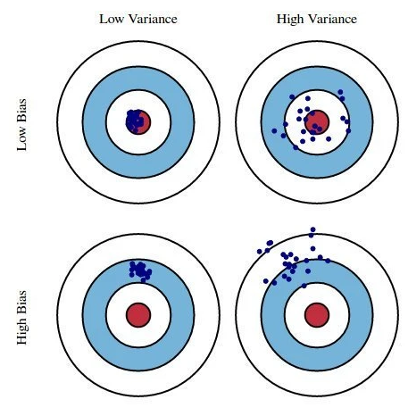
1.2.4 The Bias-variance trade-off
Overfitting leads to errors in prediction because the model fits the sample not the true relationships (data-generating process, \(f\)) between predictors and outcomes. This leads to variance in predictions for individuals depending on the sample that the model was fit within.
However, biased models also lead to errors in prediction because the model will systematically over- or under-predict (or mis-classify) outcomes for specific values of predictor(s)
Biased models are generally less complex models than the data-generating process for your outcome
Are GLMs biased models?
- GLM parmeter estimates are BLUE - best linear unbiased estimators. Parameter estimates from any sample are unbiased estimates of the linear model coefficients for population model but if DGP is not linear, this linear model will produce biased predictions.
Bias seems like a bad thing.
Both bias and variance are sources of prediction errors. They are also often inversely related (i.e., the trade-off).
Given what you know so far, why?
- Goal is to trade off a little bias for big reduction in variance to produce the most accurate predictions (and stable parameter estimates across samples for theory testing)
Useful conceptual examples of bias-variance
- Example 1: Darts from Yarkoni and Westfall (2017); They left off the most useful dartboard (* Draw on board)
- Example 2: Models (e.g. a scale) to measure individuals’ weights
1.2.5 Assessing and minimizing prediction error
- To assess prediction error, you need independent training and test datasets
- Model fit in training dataset but its fit is evaluated in single independent test set
- Use of resampling approaches like the k-fold cross-validation and bootstrap resampling
Traditional replication is NOT this. Why?
- In replication research, you obtain new data but you also fit a NEW model in these data. Ideally, you keep all the model predictors the same but you still allow coefficients to be fit to this new sample. This is a new model!
- We can minimize prediction error by using “big” data but Psychology generally does not have big data
How does big N minimize prediction error?
- Big data minimizes overfitting/model variance. You already know this for linear models from 610 as increased N leads to decreased standard errors for model parmeter estimates
- We can minimize prediction error by finding the optimal trade-off between bias and variance
- Simpler models introduce bias but reduce variance
- Regularization introduces bias but reduces variance
- Select best model from training based on its performance in test (but then need another test dataset to evaluate it!)
1.3 Concepts and Definitions (Chapters 1 & 2 in ISL)
1.3.1 An introductory framework for machine learning
Machine (Statistical) learning techniques have developed in parallel in statistics and computer science
Techniques can be coarsely divided into supervised and unsupervised approaches
Supervised approaches involve models that predict an outcome (aka: label, dependent measure, output) using predictors (aka: features, independent variables, inputs)
Unsupervised approaches involve finding structure (e.g., clusters, factors) among a set of variables without any specific outcome specified.
However supervised approaches often use unsupervised approaches in early stages as part of feature engineering
This course will focus primarily on supervised machine learning problems
What are some examples of problems/questions that require supervised approaches in your areas? and what about unsupervised?
Supervised machine learning approaches can be categorized as either regression or classification techniques
- Regression techniques involve continuous/quantitative outcomes. Regression technqiues are NOT limited to regression or the GLM. There are many more types of statitical models that are appropriate for quantitative outcomes.
- Classification techniques involve nomimal (categorical) outcomes.
- Most regression and classification techniques can handle categorical predictors
What are some examples of regression problems in your areas? and what about classification problems?
1.3.2 More details on supervised techniques
- For supervised machine learning problems we assume \(Y\) (outcome) is a function of some data generating process (DGP, \(f\)) involving a set of Xs (predictors) plus the addition of random error (\(\epsilon\)) that is independent of X and with mean of 0
\[Y = f(X) + \epsilon\]
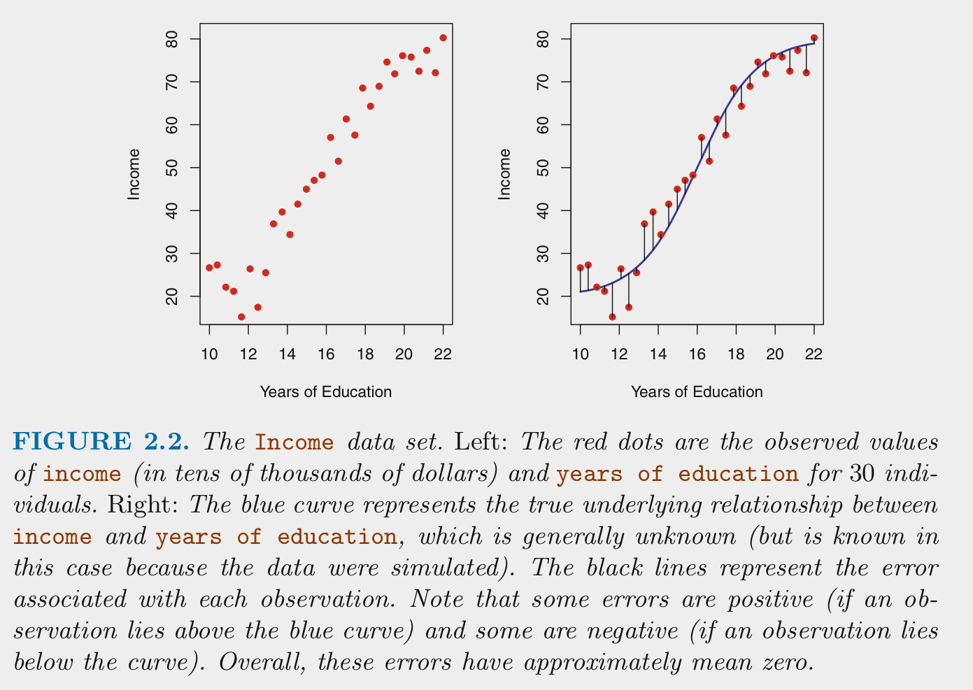
We estimate \(f\) (the DGP) for two main reasons: prediction and/or inference
\[\hat{Y} = \hat{f}(X)\] For prediction, we are most interested in the accuracy of \(\hat{Y}\) and typically treat \(\hat{f}\) as a black box
\[\hat{Y} = \hat{f}(X)\]
For inference, we are typically interested in the way that \(Y\) is affected (*) by \(X\)
- Which predictors are associated with \(Y\)
- What is the relationship between the outcome and each predictor (positive, negative, dependent on other Xs, shape of relationship such as linear or more complex)
- Does the model as a whole improve prediction beyond a null model (no predictors)
We care about good (low error) predictions even when we care about inference (we want small \(\epsilon\))
- Parameter estimates from models that dont predict well may be incorrect
- They will also be tested with low power
- Model error includes both reducible and irreducible error. If we consider both \(X\) and \(\hat{f}\) to be fixed, then
\[E(Y - \hat{Y})^2 = (f(X) + \epsilon - \hat{f}(X))^2\]
\[= [f(X) - \hat{f}(X)]^2 + Var(\epsilon)\]
- \([f(X) - \hat{f}(X)]^2\) is reducible and \(Var(\epsilon)\) is irreducible
- Irreducible error results from other important \(X\) that we fail to measure and from measurement error in \(X\) and \(Y\)
- Irreducible error serves as an (unknown) bounds for model accuracy (without collecting new X)
- Reducible error results from a mismatch between \(\hat{f}\) and the true \(f\)
- This course will focus on techniques to estimate \(f\) with the goal of minmizing reducible error
1.3.3 How do we estimate \(f\)?
We need a sample of \(n\) observations of \(Y\) and \(X\) that we will call our training data
There are two types of statistical methods that we can use for \(\hat{f}\): parametric and non-parametric methods
- Parametric methods:
- First, make an assumption about the function form or shape of \(f\).
- For example, the general linear model assumes: \(f(X) = \beta_0 + \beta_1*X_1 + \beta_2*X2 + ... + \beta_p*X_p\)
- Next, the model is fit to the training data set. In other words, the parameter estimates (e.g., \(\beta_0, \beta_1\)) are derived to minimize some cost function (e.g., mean squared error for the GLM)
- Parametric methods reduce the problem of estimating \(f\) down to one of only estimating some set of parameters for a chosen model
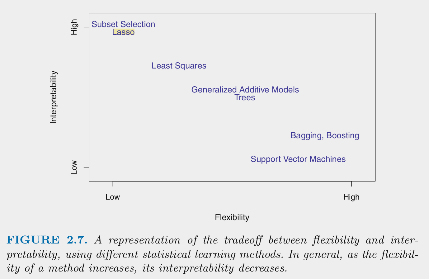
- Parametric methods often yield more interpretable models
- But they are often not very flexible. If you chose the wrong model (shape for \(\hat{f}\) that does not match \(f\)) the model will not fit well in the training data (and more importantly in new testing data either)
- First, make an assumption about the function form or shape of \(f\).
- Non-parametric methods:
- Do not make any assumption about the form/shape of \(f\)
- Can fit well for a wide variety of forms/shapes for \(f\)
- This flexibilty comes with costs
- They require larger \(n\) than parametric models
- They may overfit the training data (low error in training data but much higher error in new testing data)
- They are often less interpretable
Generally: * Flexiblity and intepretability are inversely related
- Models need to be flexible enough to fit \(f\) well
- Additional flexiblity beyond this can produce overfitting
- Parametric models are generally less flexible than non-parametric models
- Parametric models can become more flexible by increasing \(p\) (more predictors, more complex, non-linear forms for predictors)
- Parametric models can be made less flexible through regularization. There are techniques to make some non-parametric models less flexible as well
- You want the sweet spot for prediction. You may want even less flexible for inference
1.3.4 How do we assess model performance?
There is no universally best statistical method or model
- Depends on the true \(f\) and your goal (prediction or inference)
We will often compare multiple types of statistical models (various parameteric and non-parametric models) and configurations of these models (e.g., different sets of X)
When comparing models/configurations, we need to both fit these models and then select the best one
- Best needs to be defined with respect to some performance metric in new (test) data
- There are many performance metrics you might use (we will learn many)
- Root Mean squared error (RMSE) is common for regression problems
- Accuracy is common for classification problems
Two types of performance problems are typical
- Models that dont adequately represent the true \(f\) will be biased (and perform poorly in training and test data)
- However, flexible models may be overfit to the training data
- They will perform well in training but poorly in new test data
- They will show high variance such that the model changes drastically depending on the training set used
More generally, these two problems are largely inversely related
- Knows as the Bias-Variance trade-off
- We previously discused reducible and irreducible error
- Reducible error can be parsed into components due to bias and variance
1.4 An Empirical Demonstration of Overfitting and the Bias-Variance Trade-off
We will use these two packages in everything we do
Use functions regularly (reading assigned soon)
Simulations are powerful tools to help understand how analytic methods work. We will spend some time learning how to do them.
An important step in the simulation process is generating data
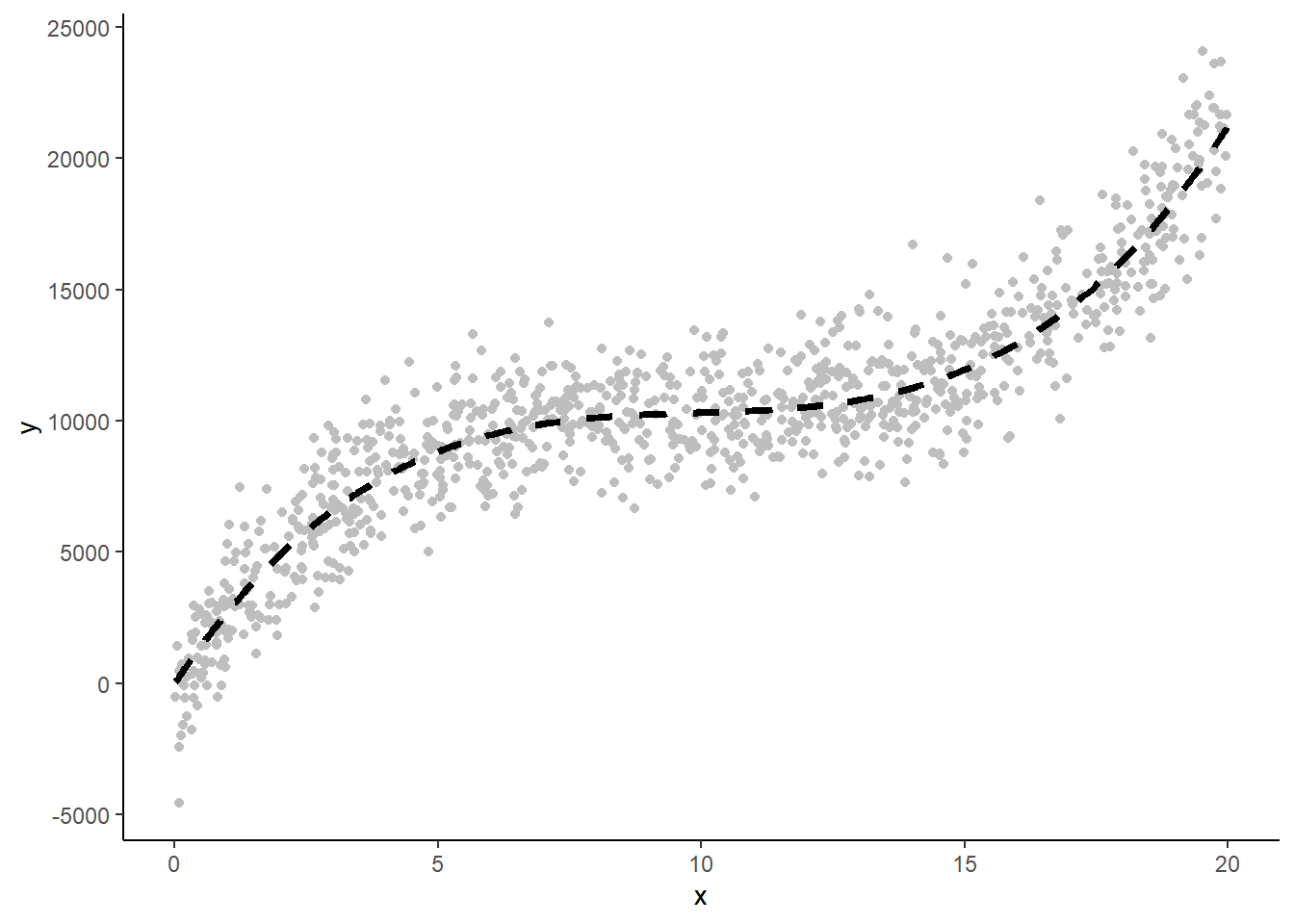
This data generating process (DGP) function uses \(rnorm()\) to generate random y as a cubic function of x with normally distributioned residuals
- See \(?rnorm\) and the CRAN task view on probability distributions for more info
get_raw_y <- function(x, noise) {
  b0 <- 10000
  b1 <- 2
  b2 <- 3
  b3 <- 10
  h <- -10
  y <- rnorm(length(x), b0 + (b1 * x) + (b2 * x^2) + (b3 * (x + h)^3), noise)
}
We will be using ggplot2 for all figures. Setting default style here. I am generally a fan of Edward Tufte’s principles about chartjunk and the data-ink ratio for visual display of data.
Alas, I am still a fan of axis lines. See also: \(geom\_rangeframe() + theme\_tufte()\) in ggthemes package
This is an example of the raw data and this cubic dgp with:
n = 1000
x = 0 - 20 from uniform distribution
noise = 1500 for raw data (0 for dgp line)
Now we:
Set up parameters for the simulation
Use set.seed() for reproducible data
Get three random samples (vs. monte carlo simulation?) of training data to fit models
- See \(?runif\) for random sampling of uniform distributions used for x
#get three random samples
train1 <- tibble(x = runif(n_train, x_min, x_max),
                 y = get_raw_y(x, noise))

train2 <- tibble(x = runif(n_train, x_min, x_max),
                 y = get_raw_y(x, noise))

train3 <- tibble(x = runif(n_train, x_min, x_max),
                 y = get_raw_y(x, noise))
Use caret package to fit, select, and evaluate/test models
\(trainControl()\) sets up general parameters used in \(train()\) to use across models (e.g., cv method, performance metric)
\(train()\) fits the specified model (and selects best model configuration if using cv)
Here we fit three types of models in each of the three different training datasets
- simple GLM
- polynomial (25th order) GLM
- polynomial lasso regression using glmnet (with lambda = 300 *)
tc_fit <- trainControl(method = "none")

glm_linear1 <- train(y ~ x, data = train1,
                     method = "glm", trControl = tc_fit)
glm_linear2 <- train(y ~ x, data = train2,
                     method = "glm", trControl = tc_fit)
glm_linear3 <- train(y ~ x, data = train3,
                     method = "glm", trControl = tc_fit)

glm_poly1 <- train(y ~ poly(x, 25), data = train1,
                   method = "glm", trControl = tc_fit)
glm_poly2 <- train(y ~ poly(x, 25), data = train2,
                   method = "glm", trControl = tc_fit)
glm_poly3 <- train(y ~ poly(x, 25), data = train3,
                   method = "glm", trControl = tc_fit)

tune_grid <- expand.grid(alpha = 1, lambda = 300)
lasso_poly1 <- train(y ~ poly(x, 25), data = train1,
                     method = "glmnet", trControl = tc_fit,
                     tuneGrid = tune_grid,
                     preProcess = c("center", "scale"))
lasso_poly2 <- train(y ~ poly(x, 25), data = train2,
                     method = "glmnet", trControl = tc_fit,
                     tuneGrid = tune_grid,
                     preProcess = c("center", "scale"))
lasso_poly3 <- train(y ~ poly(x, 25), data = train3,
                     method = "glmnet", trControl = tc_fit,
                     tuneGrid = tune_grid,
                     preProcess = c("center", "scale"))
Use \(predict()\) with caret model to get predicted values for y in train and test data sets
Notice that test set has NEW set of x and y that werent used for fitting any of the models. This allows for a test of these models that will NOT be overfit
NOTE: trimming datasets b/c of problems with high order polynomials at edge of x range
train1 <- train1 %>%
  filter(x > x_min + 1 & x < x_max - 1) %>%
  mutate(y_dgp = get_raw_y(x, 0),
         y_glm_linear = predict(glm_linear1, tibble(x)),
         y_glm_poly = predict(glm_poly1, tibble(x)),
         y_lasso_poly = predict(lasso_poly1, tibble(x)),)

train2 <- train2 %>%
  filter(x > x_min + 1 & x < x_max - 1) %>%
  mutate(y_dgp = get_raw_y(x, 0),
         y_glm_linear = predict(glm_linear2, tibble(x)),
         y_glm_poly = predict(glm_poly2, tibble(x)),
         y_lasso_poly = predict(lasso_poly2, tibble(x)),)

train3 <- train3 %>%
  filter(x > x_min + 1 & x < x_max - 1) %>%
  mutate(y_dgp = get_raw_y(x, 0),
         y_glm_linear = predict(glm_linear3, tibble(x)),
         y_glm_poly = predict(glm_poly3, tibble(x)),
         y_lasso_poly = predict(lasso_poly3, tibble(x)),)

test <- tibble(x = runif(n_test, x_min + 1, x_max - 1),
               y = get_raw_y(x, noise),
               y_dgp = get_raw_y(x, 0),
               y_glm_linear1 = predict(glm_linear1, tibble(x)),
               y_glm_linear2 = predict(glm_linear2, tibble(x)),
               y_glm_linear3 = predict(glm_linear3, tibble(x)),
               y_glm_poly1 = predict(glm_poly1, tibble(x)),
               y_glm_poly2 = predict(glm_poly2, tibble(x)),
               y_glm_poly3 = predict(glm_poly3, tibble(x)),
               y_lasso_poly1 = predict(lasso_poly1, tibble(x)),
               y_lasso_poly2 = predict(lasso_poly2, tibble(x)),
               y_lasso_poly3 = predict(lasso_poly3, tibble(x)))
Now that we have raw and predicted values in the 3 training sets and test, we can see how well the models do:
Calculate root mean square error (RMSE) for each model in its respective training set and in the independent test to index performance (i.e., the performance metric)
Average training RMSE over the three training sets to get a stable estimate (* vs. simulation vs. cv?)
Using a bigger test set to also get a stable estimate of error (*)
rmse <- crossing(model = c("train1", "train2", "train3"),
model_type = c("glm_linear", "glm_poly", "lasso_poly"),
set_type = c("train", "test")) %>%
mutate(rmse = case_when(model == "train1" & model_type == "glm_linear" & set_type == "train" ~ with(train1, RMSE(y_glm_linear, y)),
model == "train2" & model_type == "glm_linear" & set_type == "train" ~ with(train2, RMSE(y_glm_linear, y)),
model == "train3" & model_type == "glm_linear" & set_type == "train" ~ with(train3, RMSE(y_glm_linear, y)),
model == "train1" & model_type == "glm_poly" & set_type == "train" ~ with(train1, RMSE(y_glm_poly, y)),
model == "train2" & model_type == "glm_poly" & set_type == "train" ~ with(train2, RMSE(y_glm_poly, y)),
model == "train3" & model_type == "glm_poly" & set_type == "train" ~ with(train3, RMSE(y_glm_poly, y)),
model == "train1" & model_type == "lasso_poly" & set_type == "train" ~ with(train1, RMSE(y_lasso_poly, y)),
model == "train2" & model_type == "lasso_poly" & set_type == "train" ~ with(train2, RMSE(y_lasso_poly, y)),
model == "train3" & model_type == "lasso_poly" & set_type == "train" ~ with(train3, RMSE(y_lasso_poly, y)),
model == "train1" & model_type == "glm_linear" & set_type == "test" ~ with(test, RMSE(y_glm_linear1, y)),
model == "train2" & model_type == "glm_linear" & set_type == "test" ~ with(test, RMSE(y_glm_linear2, y)),
model == "train3" & model_type == "glm_linear" & set_type == "test" ~ with(test, RMSE(y_glm_linear3, y)),
model == "train1" & model_type == "glm_poly" & set_type == "test" ~ with(test, RMSE(y_glm_poly1, y)),
model == "train2" & model_type == "glm_poly" & set_type == "test" ~ with(test, RMSE(y_glm_poly2, y)),
model == "train3" & model_type == "glm_poly" & set_type == "test" ~ with(test, RMSE(y_glm_poly3, y)),
model == "train1" & model_type == "lasso_poly" & set_type == "test" ~ with(test, RMSE(y_lasso_poly1, y)),
model == "train2" & model_type == "lasso_poly" & set_type == "test" ~ with(test, RMSE(y_lasso_poly2, y)),
model == "train3" & model_type == "lasso_poly" & set_type == "test" ~ with(test, RMSE(y_lasso_poly3, y)))) %>%
group_by(model_type, set_type) %>%
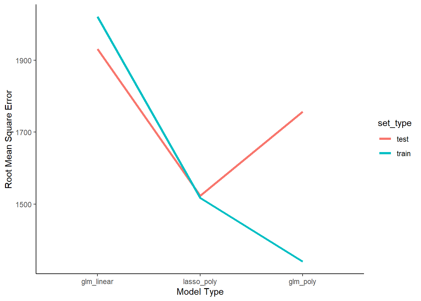
summarize(mean_rmse = mean(rmse))What do we expect about RMSE for the three models in train and test?
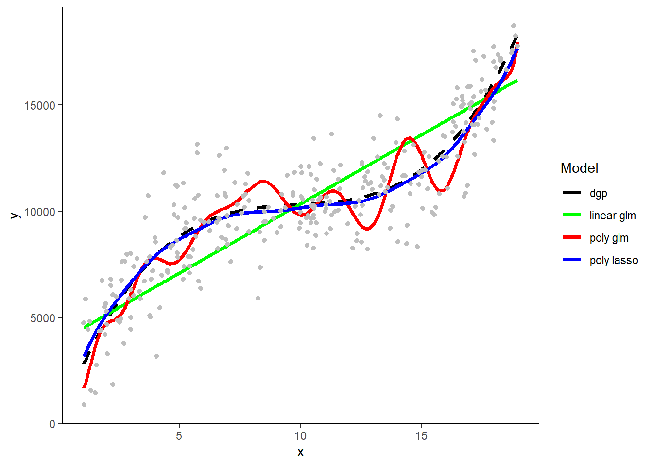
- The linear GLM is biased and wont even fit train for this reason. However, its not very flexible so it wont be overfit to train and therefore should fit comparably in test. The polynomial GLM won’t be biased at all given that the DGP is polynomial. However it is overally flexible (25th order) and so will substantially overfit the training data such that its performance will be poor in test. The polynomial lasso will be the sweet spot in bias-variance trade-off. It has a little bias but not much. However, it is not as flexible due to reguarization by lambda so it wont be overfit to train. Therefore it should do well in test.
Connect model flexibility to variance in the bias-variance trade-off? How will we see this when we look at the predicted values for models in train and test?
- A very flexible model will fit closely to the raw data in the sample within which it is trained. This means that the models will be very sample specific so that models from different samples will have very different forms (e.g., coefficients) and make very different predictions from each other when they are used in new (test) data.
Now lets start by viewing RMSE for the three model types in training and test sets
- Compare RMSE across three models within training
- Compare how RMSE changes for each model across training and test
- Compare RMSE across three models within test?
- Specifically compare performance of linear GLM with polynomial GLM
Would these observations always be the same regardless of the DGP?
- For bias, no. Absolute levels of bias would not always be the same. For example, if the DGP was linear, the linear GLM would not have much bias. Of course, the bias of the polynomial models would also be comparably low because they can fit linear relationships too. Alternatively, if the DGP was some other form (e.g., logistic), bias would be high for all of the models because none of them could represent that shape well. For variance, generally yes. The more flexible the model, the more ability it has to follow “noise” in the specific sample it is fit within. Of couse, if the specific flexibility available in the model is well aligned with the true DGP there will be less overfitting and therefore less variance across models developed in different training samples.
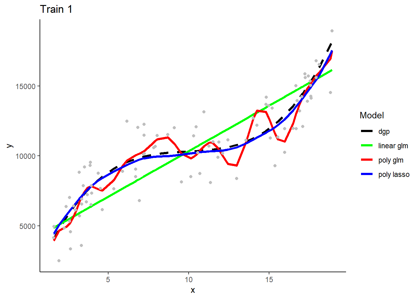
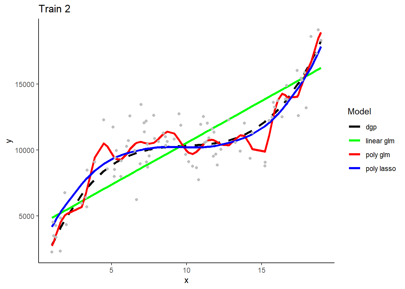
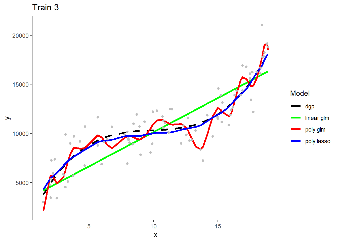
Here are the three model types’ predictions in the samples that they were fit.
What do you observe with respect to bias and variance/overfitting?
Here are predictions from the three model types when trainined in the first training sample
How is bias and variance/overfitting displayed when these models make predictions in new test data.
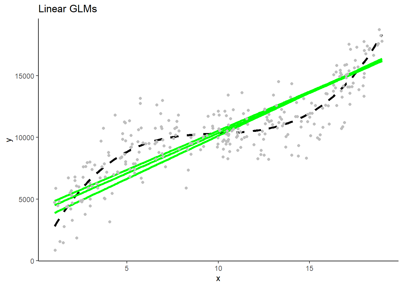
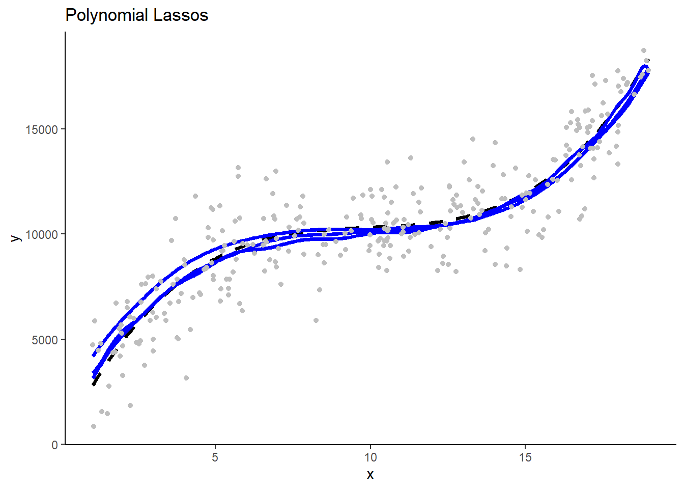
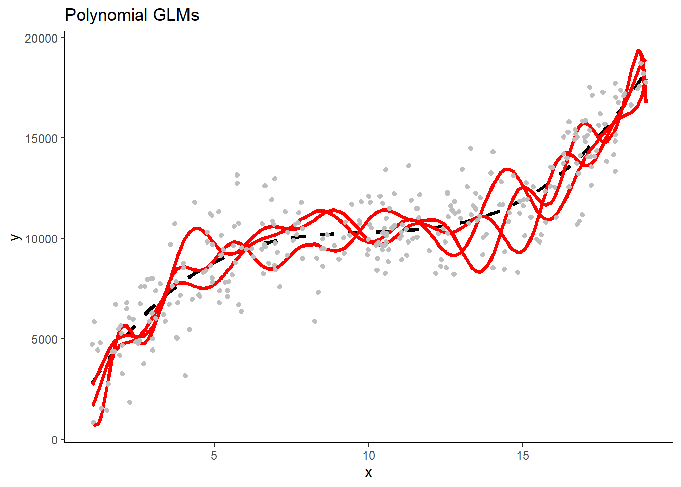
What will we see if we superimposed predictions from models fit in the other two training samples? Consider each model type separately.
- The three linear GLMS will look very similar b/c they have low variance in their fit. The three polynomial Lassos** will also look very similar. In contrast, the three polynomial GLMs will make very different predictions b/c their high flexibility/complexity relative to n) leads to high variance.
These are separate plots of predictions in the new test sample for models fit in the three separate training samples by model type. Note the impact of differences in model variance/overfit.
1.5 Programming Tips
- Consistent syntax/style is VERY important
- Use the Tidyverse
- Review Grolemund and Wickham (2016) sections 8 (Workflow: projects) and 10 (Tibbles)
- Refer to Grolemund and Wickham (2016) section 11 for read_rds() read_csv, write_rds(), and write_csv() for the homework
- See also ?file.path() in R