# set up environment.
library(tidyverse) # for general data wrangling
library(tidymodels) # for modeling
options(conflicts.policy = "depends.ok")

library(magrittr, exclude = c("set_names", "extract"))
library(xfun, include.only = "cache_rds")

source("https://github.com/jjcurtin/lab_support/blob/main/fun_eda.R?raw=true")
source("https://github.com/jjcurtin/lab_support/blob/main/fun_plots.R?raw=true")
source("https://github.com/jjcurtin/lab_support/blob/main/fun_ml.R?raw=true")
theme_set(theme_classic())
options(tibble.width = Inf)
path_data <- "./data"

rerun_setting <- FALSE IAML Unit 10: Advanced Models - Neural Networks
Learning Objectives
- What are neural networks
- Types of neural networks
- Neural network architecture
- layers and units
- weights and biases
- activation functions
- cost functions
- optimization
- epochs
- batches
- learning rate
- How to fit 3 layer MLPs in tidymodels using brulee
Introduction to Nerual Networks with brulee package
We will be using the brulee engine to fit our neural networks in tidymodels.
brulee gives us access to 3 layer (single hidden layer) and 4 layer (two hidden layer using brulee_two_layer engine) MLP neural networks. In our opinion, these are sufficient for many/most feed forward networks in the social sciences.
Yay!!
That said, the keras package provides an R Interface to the Keras API in Python.
From the website:
Keras is a high-level neural networks API developed with a focus on enabling fast experimentation. Being able to go from idea to result with the least possible delay is key to doing good research.
Keras has the following key features:
- Allows the same code to run on CPU or on GPU, seamlessly.
- User-friendly API - which makes it easy to quickly prototype deep learning models.
- Built-in support for basic multi-layer perceptrons, convolutional networks (for computer vision), recurrent networks (for sequence processing), and any combination of both.
- Supports arbitrary network architectures: multi-input or multi-output models, layer sharing, model sharing, etc. This means that Keras is appropriate for building essentially any deep learning model, from a memory network to a neural Turing machine.
Keras is actually a wrapper around an even more extensive open source platform, TensorFlow, which has also been ported to the R environment
TensorFlow is an end-to-end open source platform for machine learning. It has a comprehensive, flexible ecosystem of tools, libraries and community resources that lets researchers push the state-of-the-art in ML and developers easily build and deploy ML powered applications.
TensorFlow was originally developed by researchers and engineers working on the Google Brain Team within Google’s Machine Intelligence research organization for the purposes of conducting machine learning and deep neural networks research
Tidymodels does provide an interface to keras but its not that good and brulee is much better.
However, if you need the power of Keras for more complicated models (more than 2 hidden layers, more complex configurations like recursive networks, etc) you might start with this book to learn how to use Keras directly in R outside of tidymodels.
Getting keras set up can take a little bit of upfront effort.
We provide an appendix to guide you through this process
But we think brulee inside of tidymodels will likely meet many of your needs
Setting up our Environment
Now lets get started
The MNIST dataset
The MNIST database (Modified National Institute of Standards and Technology database) is a large database of handwritten digits that is commonly used for training and testing in the field of machine learning.
It consists of two sets:
- There are 60,000 images from 250 people in train
- There are 10,000 images from a different 250 people in test (from different people than in train)
Each observation in the datasets represent a single image and its label
- Each image is a 28 X 28 grid of pixels = 784 predictors (x1 - x784)
- Each label is the actual value (0-9; y). We will treat it as categorical because we are trying to identify each number “category”, predicting a label of “4” when the image is a “5” is just as bad as predicting “9”
Let’s start by reading train and test sets
data_trn <- read_csv(here::here(path_data, "mnist_train.csv.gz"),
                     col_types = cols()) |>
  mutate(y = factor(y, levels = 0:9, labels = 0:9))
data_trn |> dim()
[1] 60000 785data_test <- read_csv(here::here(path_data, "mnist_test.csv"),
col_types = cols()) |>
mutate(y = factor(y, levels = 0:9, labels = 0:9))
data_test |> dim()[1] 10000 785Here is some very basic info on the outcome distribution
- in train
# A tibble: 10 × 3
   y         n   prop
   <fct> <int>  <dbl>
 1 0      5923 0.0987
 2 1      6742 0.112
 3 2      5958 0.0993
 4 3      6131 0.102
 5 4      5842 0.0974
 6 5      5421 0.0904
 7 6      5918 0.0986
 8 7      6265 0.104
 9 8      5851 0.0975
10 9      5949 0.0992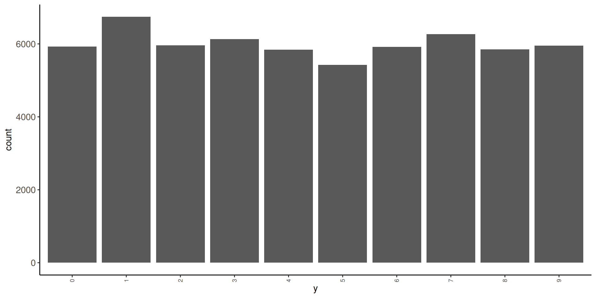
- in test
# A tibble: 10 × 3
   y         n   prop
   <fct> <int>  <dbl>
 1 0       980 0.098
 2 1      1135 0.114
 3 2      1032 0.103
 4 3      1010 0.101
 5 4       982 0.0982
 6 5       892 0.0892
 7 6       958 0.0958
 8 7      1028 0.103
 9 8       974 0.0974
10 9 1009 0.101 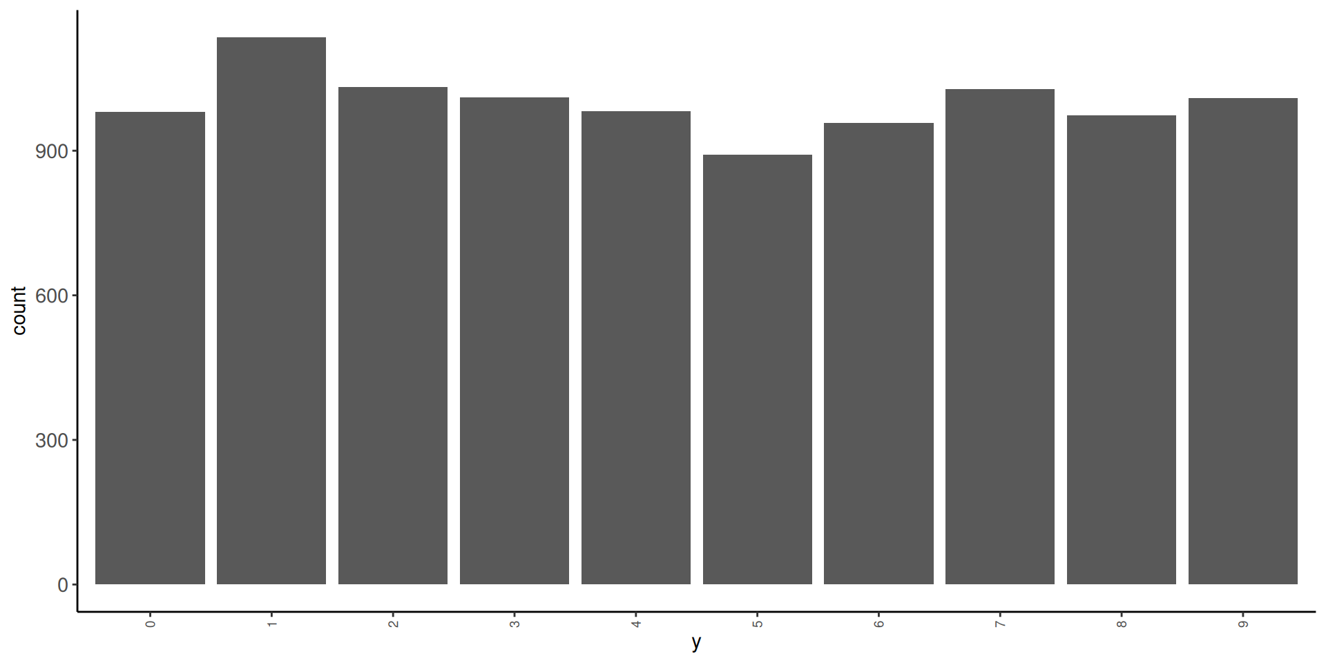
Let’s look at some of the images. We will need a function to display these images. We will use as.cimg() from the imager package
Observations 1, 3, 10, and 100 in training set


And here is the first observation in test set

Let’s understand the individual predictors a bit more
- Each predictor is a pixel in the 28 X 28 grid for the image
- Pixel intensity is coded for intensity in the range from 0 (black) to 255 (white)
- First 28 variables are the top row of 28 pixels
- Next 28 variables are the second row of 28 pixels
- There are 28 rows of 28 predictors total (784 predictors)
- Lets understand this by changing values for individual predictors
- Here is the third image again
What will happen to the image if I change the value of predictor x25 to 255

- Change the
x25to 255

What will happen to the image if I change the value of predictor x29 to 255
- Change the
x29to 255

What will happen to the image if I change the value of predictor x784 to 255
- Change the
x784to 255

Fitting Neural Networks
Let’s train some models to understand some basics about neural networks and the use of brulee within tidymodels
We will fit some configurations in the full training set and evaluate their performance in test
We are NOT using test to select among configurations (it wouldn’t be a true test set then) but only for instructional purposes.
We will start with an absolute minimal recipe and mostly defaults for the statistical algorithm
We will build up to more complex (and better) configurations
We will end with a demonstration of the use of the single validation set approach to select among model configurations
The default activation for the hidden units when using brulee through tidymodels is relu not sigmoid as per the basic models discussed in the book and videos.
- The activation for the output layer will always be
softmaxfor classification problems when using brulee through tidymodels- This is likely a good choice
- It provides scores that function like probabilities for each categorical response
- The activation for the output layer will always be ‘linear’ for regression problems.
- Also a generally good choice
- The hidden units can have a variety of different activation functions. These are the options for hidden units in brulee
There are a number of points in the fitting process for neural networks where random numbers needed
- initializing weights for hidden and output layers
- selecting units for
dropout - selecting batches within epochs
- allocation between train and validation for early stopping
If you want these steps to be reproducible, you should set a seed before fitting the model. We will do that for all our models below using the same seed each time
Let’s start with a minimal recipe
- 10 level categorical outcome as factor
- Will be used to establish 10 output neurons
Here are feature matrices for train and test using this recipe
Lets set up a 3 layer (one hidden layer) as per the book and videos
Lets start with a configuration that approximates the basic models we have been discussing in the book and videos (with a few parameters set to their defaults in brulee rather than the defaults in the book and videos).
Some of these are NOT the defaults for brulee in tidymodels so we will explicitly set them either inside of mlp() or set_engine()
We will show defaults for these arguments when we override them. Most of these defaults as sensible places to start BUT they should all likely be considered for tuning if you want the best performance!
For more details about the many arguments that can be explored (and their default values) see the following documetation
- https://parsnip.tidymodels.org/reference/mlp.html
- https://parsnip.tidymodels.org/reference/details_mlp_brulee.html
- https://parsnip.tidymodels.org/reference/details_mlp_brulee_two_layer.html
- https://brulee.tidymodels.org/
Let’s fit this first model configuration in training set
set.seed(1234567)
fit_1 <- mlp(activation = "sigmoid",   # from book, default in brulee = "relu"
             epochs = 30, # default = 100 (set to 30 to speed things up for now)
             hidden_units = 3, # default = 3,
             learn_rate = 0.01, # default = .01
             penalty = 0,  # from book, default = .001 (and mixture defaults to 0)
             dropout = 0) |>   # from book, default = 0
    set_mode("classification") |>
    set_engine("brulee",
               verbose = TRUE,    # default = FALSE (output loss for each epoch)
               validation = 0,    # from book, default = .1 (if 0, calculate loss in training)
               stop_iter = 5) |>  # default = 5 (stop early after loss increases this many times)
    fit(y ~ ., data = feat_trn)
Here is this model’s performance in test
It’s not that great but not horrible (What would you expect by chance?)
Theoretically, the scale of the inputs should not matter
HOWEVER, gradient descent works better with inputs on the same scale
We will also want inputs with the same variance if we later apply L2 regularization to our models
- There is a lot of discussion about how best to scale inputs
- Best if the input means are near zero
- Best if variances are comparable
We could:
- Use
step_normalize()[Bad choice of function names by tidymodel folks; standardize vs. normalize] - Use
step_range() - Book range corrected based on known true range (
/ 255)
We will use step_normalize()
This is wrong! Luckily we glimpsed our feature matrix (not displayed here)
Question: What went wrong and what should we do?
Many of the features have zero variance b/c they are black for ALL of the images (e.g., top rows of pixels. We can not scale a predictor with zero variance b/c when we divide by the SD = 0, we get NaN). At a minimum, we should remove zero variance predictors in training from training and test
For example
Let’s remove zero variance predictors before we scale
- To be clear, zero variance features are NOT a problem for neural networks (though clearly they won’t help either).
- But they WILL definitely cause problems for some scaling transformations.
We now have 717 (+ y) features rather than 28 * 28 = 784 features
Let’s also make the feature matrix for test. This will exclude features that were zero variance in train and scale them by their mean and sd in train
Let’s fit and evaluate this new feature set with no other changes to the model configuration
set.seed(1234567)
fit_2 <- mlp(activation = "sigmoid",   # from book, default in brulee = "relu"
             epochs = 30, # default = 100 (set to 30 to speed things up for now)
             hidden_units = 3, # default = 3,
             learn_rate = 0.01, # default = .01
             penalty = 0,  # from book, default = .001 (and mixture defaults to 0)
             dropout = 0) |>   # from book, default = 0
    set_mode("classification") |>
    set_engine("brulee",
               verbose = TRUE,    # default = FALSE (output loss for each epoch)
               validation = 0,    # from book, default = .1 (if 0, calculate loss in training)
               stop_iter = 5) |>  # default = 5 (stop early after loss increases this many times)
fit(y ~ ., data = feat_trn)- That helped a LOT
- Still could be better though (but it always impresses me! ;-)
There are many other recommendations about feature engineering to improve the inputs
These include:
- Normalize (and here I mean true normalization; e.g.,
step_BoxCox(),step_YeoJohnson()) - De-correlate (e.g.,
step_pca()but retain all features?)
You can see some discussion of these issues here and here to get you started. The paper linked in the stack overflow response is also a useful starting point.
Some preliminary modeling EDA on my part suggested these additional considerations didn’t have major impact on the performance of our models with this dataset so we will stick with just scaling the features.
It is not surprising that a model configuration with only one hidden layer and 5 units isn’t sufficient for this complex task
Let’s try 30 units (cheating based on the book chapter!! ;-)
set.seed(1234567)
fit_3 <- mlp(activation = "sigmoid",   # from book, default in brulee = "relu"
             epochs = 30, # default = 100 (set to 30 to speed things up for now)
             hidden_units = 30, # default = 3,
             learn_rate = 0.01, # default = .01
             penalty = 0,  # from book, default = .001 (and mixture defaults to 0)
             dropout = 0) |>   # from book, default = 0
    set_mode("classification") |>
    set_engine("brulee",
               verbose = TRUE,    # default = FALSE (output loss for each epoch)
               validation = 0,    # from book, default = .1 (if 0, calculate loss in training)
               stop_iter = 5) |>  # default = 5 (stop early after loss increases this many times)
fit(y ~ ., data = feat_trn)- Bingo! Much, much better!
- We could see if even more units works better still but I won’t follow that through here for sake of simplicity
The Three Blue 1 Brown videos had a brief discussion of the relu activation function.
Let’s see how to use other activation functions and if this one helps.
set.seed(1234567)
fit_4 <- mlp(activation = "relu",   # default in brulee = "relu"
             epochs = 30, # default = 100 (set to 30 to speed things up for now)
             hidden_units = 30, # default = 3,
             learn_rate = 0.01, # default = .01
             penalty = 0,  # from book, default = .001 (and mixture defaults to 0)
             dropout = 0) |>   # from book, default = 0
    set_mode("classification") |>
    set_engine("brulee",
               verbose = TRUE,    # default = FALSE (output loss for each epoch)
               validation = 0,    # from book, default = .1 (if 0, calculate loss in training)
               stop_iter = 5) |>  # default = 5 (stop early after loss increases this many times)
fit(y ~ ., data = feat_trn)Dealing with Overfitting
As you might imagine, given the number of weights to be fit in even a modest neural network (our 30 hidden unit network has 21,850 parameters to estimate), it is easy to become overfit
- 21,540 for hidden layer (717 * 30 weight + 30 biases)
- 310 for output layer (30 * 10 weights, + 10 biases)
parsnip model object

Multilayer perceptron

relu activation,
30 hidden units,
21,850 model parameters
60,000 samples, 717 features, 10 classes
class weights 0=1, 1=1, 2=1, 3=1, 4=1, 5=1, 6=1, 7=1, 8=1, 9=1
dropout proportion: 0
batch size: 60000
learn rate: 0.01
training set loss after 30 epochs: 0.0747
This will be an even bigger problem if you aren’t using “big” data
There are a number of different methods available to reduce potential overfitting
- Simplify the network architecture (fewer units, fewer layers)
- L1 and L2 regularization (including mixtures of both penalties)
- Dropout
- Early stopping by monitoring validation error to prevent too many epochs
Regularization or Weight Decay
L1 and L2 regularization is implemented in essentially the same fashion as you have seen it previously (e.g., glmnet)
The cost function is expanded to include a penalty based on the sum of the absolute value or squared weights multiplied by \(\lambda\).
In the tidymodels implementation of brulee:
- \(\lambda\) is called
penaltyand is set and/or (ideally) tuned via thepenaltyargument inmlp().- \(penalty\) = .001 is the default in brulee
penalty = 0means no regularization- Common values for the
penaltyto tune a neural network are often on a logarithmic scale between 0 and 0.1, such as 0.1, 0.001, 0.0001, etc.
- \(mixture\) is used to blend L1 and L2 (\(mixture\) = 1 for L1, = 0 for L2, and intermediate values for blends)
- \(mixture\) = 0 (L2) is default
- Here is a starting point for more reading on regularization in neural networks
Let’s set penalty = .001.
We are setting it explicitly below for clarity but since it is the default, this is the default behavior you would get if you did not include the penalty argument in mlp()
set.seed(1234567)
fit_5 <- mlp(activation = "relu",   #  default in brulee = "relu"
             epochs = 30, # default = 100 (set to 30 to speed things up for now)
             hidden_units = 30, # default = 3,
             learn_rate = 0.01, # default = .01
             penalty = .001,  #  default = .001 (and mixture defaults to 0)
             dropout = 0) |>   # from book, default = 0
    set_mode("classification") |>
    set_engine("brulee",
               verbose = TRUE,    # default = FALSE (output loss for each epoch)
               validation = 0,    # from book, default = .1 (if 0, calculate loss in training)
               stop_iter = 5) |>  # default = 5 (stop early after loss increases this many times)
fit(y ~ ., data = feat_trn)- Looks like there is not much benefit to regularization for this network (though we could explore other values via tuning)
- Would likely provide much greater benefit in smaller N contexts or with more complicated model architectures (more hidden units, more hidden unit layers).
NOTE: I suspect that there is a bug in the implementation of penalty. I intend to submit a reprex to confirm this. Stay tuned!!
Dropout
Dropout is a second technique to minimize overfitting.
Here is a clear description of dropout from a blog post on the Machine Learning Mastery:
Dropout is a technique where randomly selected neurons are ignored during training. They are “dropped-out” randomly. This means that their contribution to the activation of downstream neurons is temporally removed on the forward pass and any weight updates are not applied to the neuron on the backward pass.
As a neural network learns, neuron weights settle into their context within the network. Weights of neurons are tuned for specific features providing some specialization. Neighboring neurons come to rely on this specialization, which if taken too far can result in a fragile model too specialized to the training data.
You can imagine that if neurons are randomly dropped out of the network during training, that other neurons will have to step in and handle the representation required to make predictions for the missing neurons. This is believed to result in multiple independent internal representations being learned by the network.
The effect is that the network becomes less sensitive to the specific weights of neurons. This in turn results in a network that is capable of better generalization and is less likely to overfit the training data.
For further reading, you might start with the 2014 paper by Srivastava, et al that proposed the technique.
In tidymodels, you can set or tune the amount of dropout via the dropout argument in mlp()
- Srivastava, et al suggest starting with values around .5.
- You might consider a range between .1 and .5
droppout = 0(the default) means no dropout- In tidymodels implementation of brulee, you can use a non-zero
penaltyordropoutbut not both.- If you set a dropout explicitly, penalty will be set to 0 implicitly.
- if you explicitly set both to non-zero, it will generate an error.
Let’s try dropout = .1.
set.seed(1234567)
fit_6 <- mlp(activation = "relu",   #  default in brulee = "relu"
             epochs = 30, # default = 100 (set to 30 to speed things up for now)
             hidden_units = 30, # default = 3,
             learn_rate = 0.01, # default = .01
             penalty = 0,  #  default = .001 (and mixture defaults to 0)
             dropout = 0.1) |>   # from book, default = 0
    set_mode("classification") |>
    set_engine("brulee",
               verbose = TRUE,    # default = FALSE (output loss for each epoch)
               validation = 0,    # from book, default = .1 (if 0, calculate loss in training)
               stop_iter = 5) |>  # default = 5 (stop early after loss increases this many times)
fit(y ~ ., data = feat_trn)- Looks like dropout hurt rather than helped. Of course, we may have just selected a bad choice for the amount of dropout. This should be explored further and compared to what we can do using a L1 or L2 penalty instead.
- Would likely provide much greater benefit in smaller N contexts or with more complicated model architectures (more hidden units, more hidden unit layers).
Number of Epochs and Early Stopping
We have a model that is working well (fit_4)
Now lets return to the issue of number of epochs
- Too many epochs can lead to overfitting
- Too many epochs also just slow things down (not a bit deal if using GPU or overnight but still…..)
- Too few epochs can lead to under-fitting (which also produces poor performance)
- The default of
epochs = 100seems high to may and would take > ~30x longer to train than what we have been using (30 epochs).- It was likely set to that because the brulee default is to use early stopping.
- Lets see what happens if we set epochs to 100 but also turn on early stopping by checking loss in a validation set
Let’s see this in action in the best model configuration without regularization or dropout
Early stopping will be invoked if the error increases on some specified number of trials (default is stop_iter = 5)
However, this will never happen if you are using training error because training error will never increase because does not include error due to overfitting
Validation error is what you need to monitor if you want to detect overfitting
- Validation error will increase when the model becomes overfit to training
- We can have tidymodels hold back some portion of the training data for validation
validation= .1 is the default- We pass it in as an optional argument in
set_engine() - This can allow us to stop training once the model starts to become overfit to training
set.seed(1234567)
fit_7 <- mlp(activation = "relu",   # default in brulee = "relu"
             epochs = 100, # default = 100
             hidden_units = 30, # default = 3,
             learn_rate = 0.01, # default = .01
             penalty = 0,  # from book, default = .001 (and mixture defaults to 0)
             dropout = 0) |>   # from book, default = 0
    set_mode("classification") |>
    set_engine("brulee",
               verbose = TRUE,    # default = FALSE (output loss for each epoch)
               validation = 0.1,    # default = .1 (if 0, calculate loss in training)
               stop_iter = 5) |>  # default = 5 (stop early after loss increases this many times)
fit(y ~ ., data = feat_trn)This stops after 23 epochs yet fits almost identical to our model trained over 30 epochs.
It saves substantial time vs. training over 100 epochs
It might have even fit better than without early stopping if we had let the model become even more overfit but setting epochs to 100 without early stopping (we were only using 30 epochs)
Using Resampling to Select Best Model Configuration
Developing a good network architecture and considering feature engineering options involves experimentation
- We need to evaluate configurations with a valid method to evaluate performance
- validation split metric
- k-fold metric
- bootstrap method
- Each can be paired with
fit_resamples()ortune_grid()
- We need to be systematic
tune_grid()helps with this too- recipes can be tuned as well (outside the scope of this course)
Here is an example where we can select among many model configurations that differ across multiple network characteristics
- Evaluate with validation split accuracy
- Sample size is relatively big so we have 10,000 validation set observations. Should offer a low variance performance estimate
- K-fold and bootstrap would still be better but big computation costs (too big for this web book but could be done in real life!)
Its really just our normal workflow at this point
- Get splits (validation splits in this example)
Set up grid of hyperparameter values
we haven’t considered learning rate yet but that matters too as discussed in the book/videos so lets tune it
- Use
tune_grid()to fit models in training and predict into validation set for each combination of hyperparameter values
fits_nn <- cache_rds(
  expr = {
    mlp(hidden_units = tune(),
        learn_rate = tune(),
        activation = "relu",
        penalty = 0,
        dropout = 0,
        epochs = 100) |>
    set_mode("classification") |>
    set_engine("brulee",
               verbose = FALSE,
               validation = .1,
               stop_iter = 5) |>
    tune_grid(preprocessor = rec_scaled,
                  grid = grid_mlp,
                  resamples = splits_validation,
                  metrics = metric_set(accuracy))
  },
  rerun = rerun_setting,
  dir = "cache/010/",
file = "fits_nn")- Find model configuration with best performance in the held-out validation set
# A tibble: 5 × 8
  hidden_units learn_rate .metric  .estimator  mean     n std_err
         <dbl>      <dbl> <chr>    <chr>      <dbl> <int>   <dbl>
1          100       1    accuracy multiclass 0.966     1      NA
2          100       0.1  accuracy multiclass 0.966     1      NA
3           50       1    accuracy multiclass 0.960     1      NA
4           30       1    accuracy multiclass 0.957     1      NA
5          100       0.01 accuracy multiclass 0.954     1      NA
  .config
  <chr>
1 Preprocessor1_Model24
2 Preprocessor1_Model23
3 Preprocessor1_Model20
4 Preprocessor1_Model16
5 Preprocessor1_Model22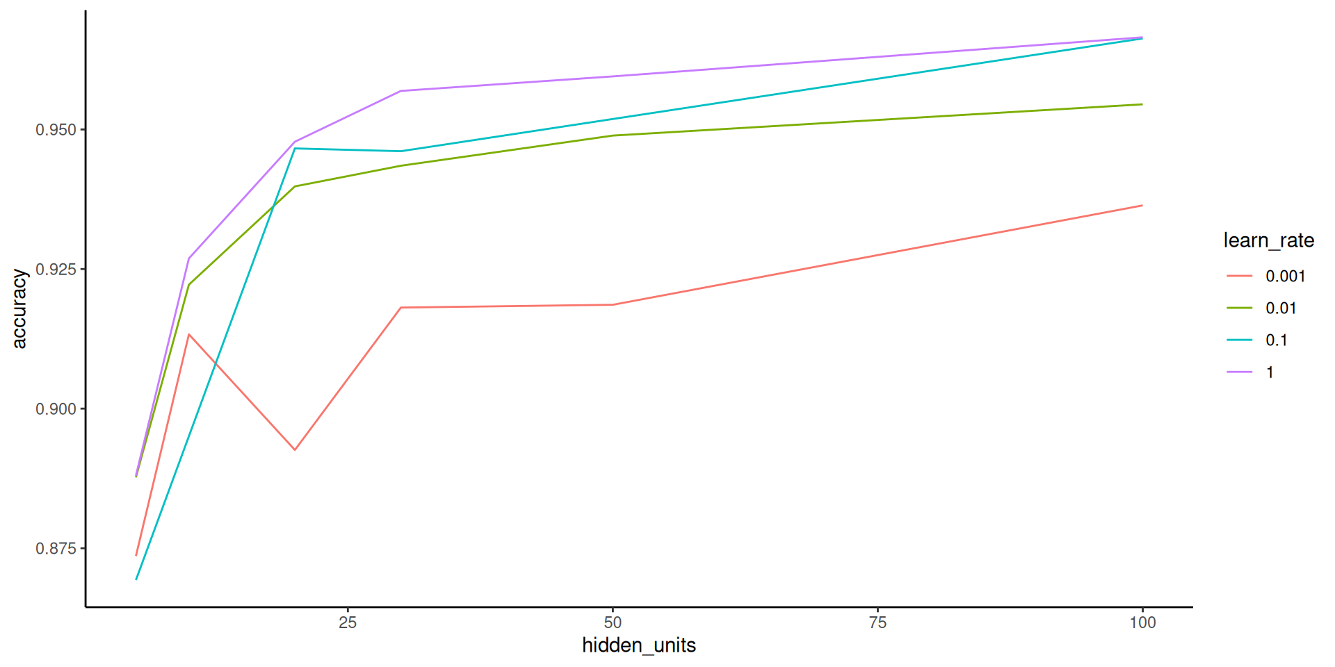
Looking at this hyperparameter plot, we might want to consider even higher number of hidden units and a higher learning rate!