IAML Unit 8: Discussion

Announcements

Confusion matrix

Ground Truth
Prediction Positive Negative
Positive TP FP
Negative FN TN

Definitions:

  • TP: True positive

  • TN: True negative

  • FP: False positive (Type 1 error/false alarm)

  • FN: False negative (Type 2 error/miss)

  • More generally

    • define accuracy, sens, spec, ppv, npv, bal_accuracy, f1
    • Cost of FP and FN?
    • How to choose between?
Ground Truth
Prediction Positive Negative
Positive 95 5
Negative 5 95
Ground Truth
Prediction Positive Negative
Positive 95 50
Negative 5 950
  • Predicting lapses
  • COVID testing during pandemic early vs. late

Resampling

  • Options?
  • similarities and differences, relative comparisons?
  • resampling held-in but not held-out. Why?
  • Why does it work?

ROC

  • Axes and various names/representations
library(tidyverse)
theme_set(theme_classic()) 
source("https://github.com/jjcurtin/lab_support/blob/main/format_path.R?raw=true")
path_models <-"~/mnt/standard/risk/models/ema" # format_path("studydata/risk/models/ema", "restricted")
preds_hour<- read_rds(file.path(path_models, 
                               "outer_preds_1hour_0_v5_nested_main.rds"))
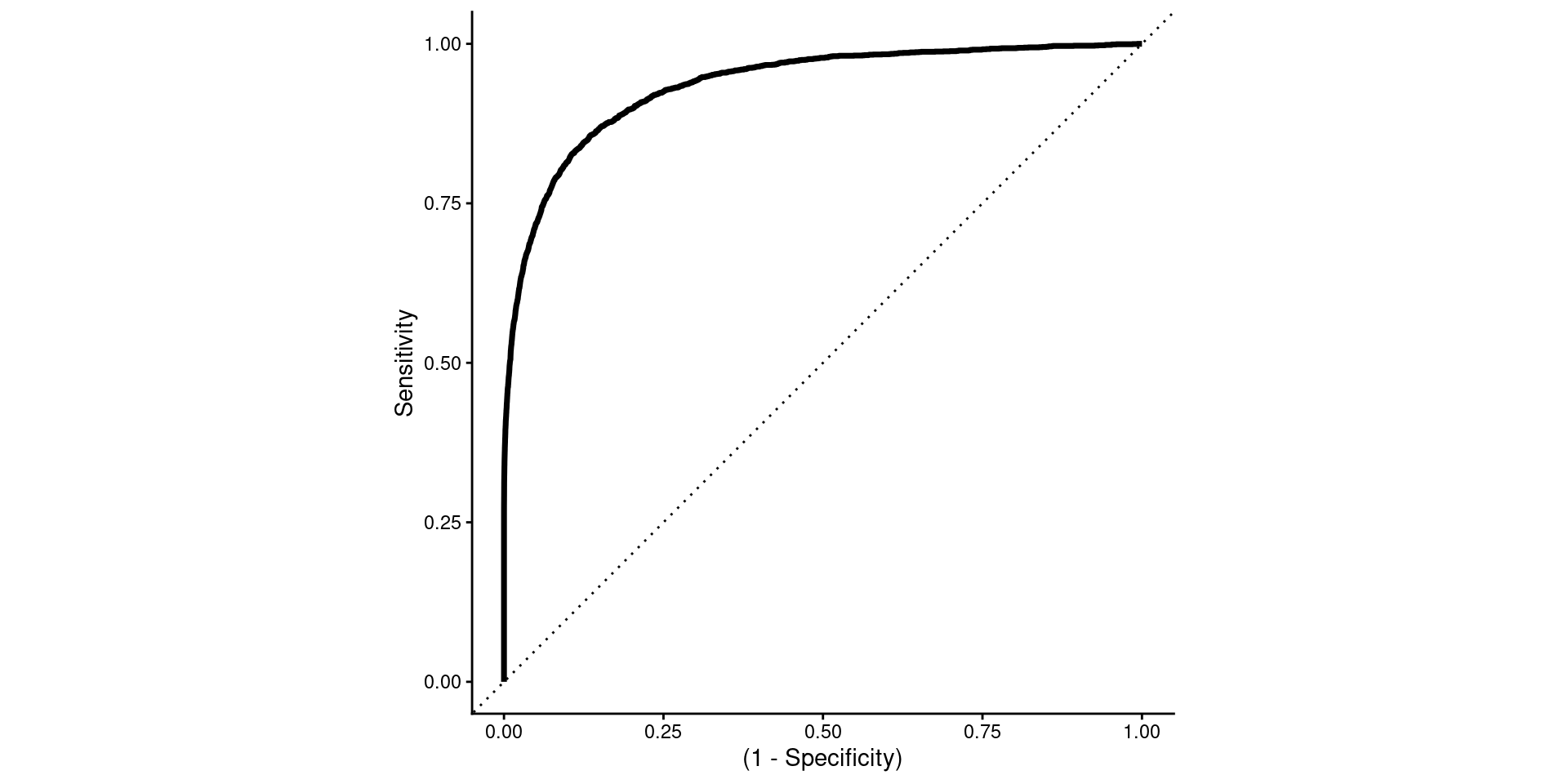
roc_hour <- preds_hour|> 
  yardstick::roc_curve(prob_beta, truth = label)

Option 1 - Sensitivity vs. 1 - Specificity

  • More common terms
  • 1 - Specificity is confusing!
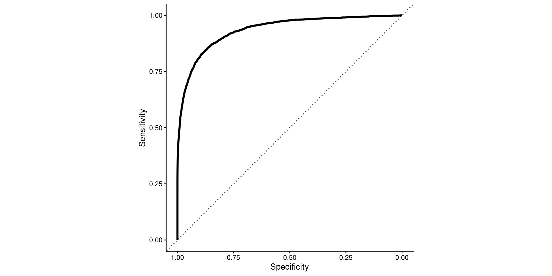
roc_hour |> 
  ggplot(aes(x = 1 - specificity, y = sensitivity)) +
    geom_path(linewidth = 1.25) +
    geom_abline(lty = 3) +
    coord_fixed(xlim = c(0, 1), ylim = c(0, 1)) +
    labs(x = "(1 - Specificity)",
        y = "Sensitivity") +
  scale_x_continuous(breaks = seq(0,1,.25))

Option 2

  • More common terms
  • Sensible (though reversed) axis
  • My preferred format
roc_hour |> 
  ggplot(aes(x = 1 - specificity, y = sensitivity)) +
    geom_path(linewidth = 1.25) +
    geom_abline(lty = 3) +
    coord_fixed(xlim = c(0, 1), ylim = c(0, 1)) +
    labs(x = "Specificity",
        y = "Sensitivity") +
  scale_x_continuous(breaks = seq(0,1,.25),
    labels = sprintf("%.2f", seq(1,0,-.25)))

Option 3 - TPR vs. FPR

  • sensible axes
  • Less common terms
  • But coming to prefer (depending on audience)
roc_hour |> 
  ggplot(aes(x = 1 - specificity, y = sensitivity)) +
    geom_path(linewidth = 1.25) +
    geom_abline(lty = 3) +
    coord_fixed(xlim = c(0, 1), ylim = c(0, 1)) +
    labs(x = "False Positive Rate (FPR)",
        y = "True Positive Rate (TPR)") +
  scale_x_continuous(breaks = seq(0,1,.25))

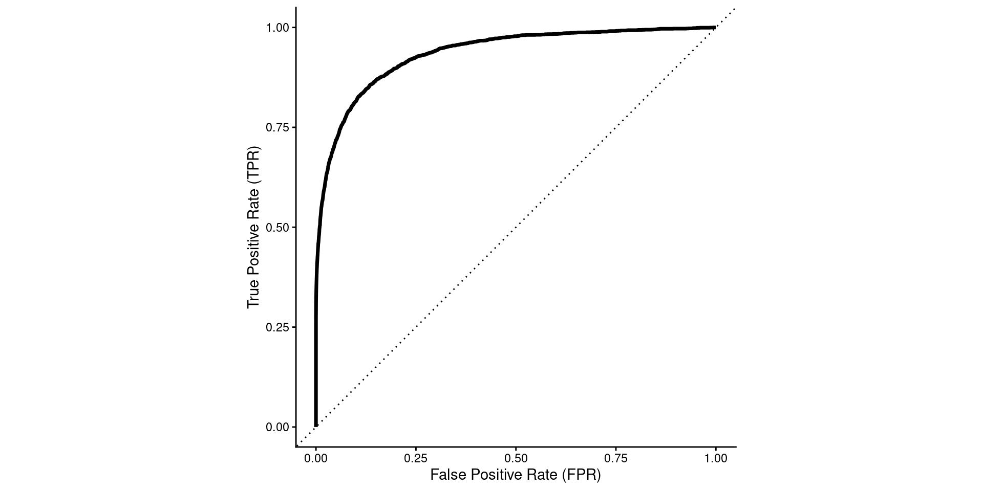
  • Why is top right perfect performance
  • Thresholds
  • Interpretation of auROC and the diagonal line
  • Can we go over some more concrete (real-world) examples of when it would be a good idea to use a different threshold for classification?
  • Are there any techniques to optimize decision thresholds? Or is it trial and error.
  • How does AUROC perform in highly imbalanced datasets
  • Sensitivity vs. Specificity Trade-offs, is it always true increase in one will sacrifice the other
roc_hour |> 
  ggplot(aes(x = 1 - specificity, y = sensitivity)) +
    geom_path(linewidth = 1.25) +
    geom_abline(lty = 3) +
    coord_fixed(xlim = c(0, 1), ylim = c(0, 1)) +
    labs(x = "Specificity",
        y = "Sensitivity") +
  scale_x_continuous(breaks = seq(0,1,.25),
    labels = sprintf("%.2f", seq(1,0,-.25)))

  • “means” of sensitivity/specificity vs. precision(ppv)/recall(sensitivity)
  • Balanced accuracy is the arithmetic mean of sens/spec
  • f1 is the harmonic mean of precision/recall

harmonic mean example: if a vehicle travels 60km outbound at a speed of 60 km/h and returns the same distance at a speed of 20 km/h, then its average speed is the harmonic mean of x and y (30 km/h), not 40 km/h

harmonic mean of

  • .5 and .5 is .5
  • .75 and .75 is .75
  • .25 and .75 is .375
  • 0 and 1 is 0

Kappa

  • expected accuracy
    • given majority class proportion
    • by chance given base rates
  • ratio of improvement above expected accuracy